Pore-Scale Modeling of Navier-Stokes Flow in Distensible Networks and Porous Media

Taha Sochi

Nomenclature

αcorrection factor for axial momentum flux

βstiffness coefficient in pressure-area relation

κviscosity friction coefficient

μfluid dynamic viscosity

νfluid kinematic viscosity

ρfluid mass density

?Poisson’s ratio of tube wall

Atube cross sectional area

Aintube cross sectional area at inlet

Aotube cross sectional area at reference pressure

Aoutube cross sectional area at outlet

EYoung’s elastic modulus of tube wall

fflow continuity residual function

hovessel wall thickness at reference pressure

J Jacobian matrix

Ltube length

nnumber of network nodes

N norm of residual vector

ppressure

p pressure vector

piinlet pressure

pooutlet pressure

?p pressure perturbation vector

Qvolumetric flow rate

rflow continuity residual

r residual vector

Rtube radius

ttime

xtube axial coordinate

1 Introduction

There are many scientific,industrial and biomedical applications related to the flow of fluids in distensible networks of interconnected tubes and compliant porous materials.A few examples are magma migration,microfluidic sensors,fluid filtering devices,deformable porous geological structures such as those found in petroleum reservoirs and aquifers,as well as almost all the biological flow phenomena like blood circulation in the arterial and venous vascular trees or biological porous tissue and air movement in the lung windpipes.

There have been many studies in the past related to this subject[Whitaker(1986);Spiegelman(1993);Chenet al(2000);Ambrosi(2002);Formaggia,Lamponi and Quarteroni(2003);Krenz and Dawson(2003);Klubertanzet al(2003);Mabotuwana,Cheng and Pullan(2007);Nobile(2009);Ju,Wu and Fan(2011)];however most of these studies are based on complex numerical techniques built on tortuous mathematical infrastructures which are not only difficult to implement with expensive computational running costs,but are also difficult to verify and validate.The widespread approach in modeling the flow in deformable structures is to use the one-dimensional Navier-Stokes finite element formulation for modeling the flow in networks of compliant large tubes[Formaggia,Lamponi and Quarteroni(2003);Sochi(2013a)]and the extended Darcy formulation for the flow in deformable porous media which is based on the poromechanics theory or some similar numerical meshing techniques[Huygheet al(1992);Coussy(2004,2010);Chapelleet al(2010)].Rigid network flow models,like Poiseuille,may also be used as an approximation although in most cases this is not really a good one[Sochi(2013b)].There have also been many studies in the past related to the flow of fluids in ensembles of interconnected ducts using pore-scale network modeling especially in the earth science and petroleum engineering disciplines[Sorbie,Clifford and Jones(1989);Sorbie(1990,1991);Valvatne(2004);Sochi(2007,2009,2010a)].However,there is hardly any work on the use of pore-scale network modeling to simulate the flow of fluids in deformable structures with distensible characteristics such as elastic or viscoelastic mechanical properties.

There are several major advantages in using pore-scale network modeling over the more traditional analytical and numerical approaches.These advantages include a comparative ease of implementation,relatively low computational cost,reliability,robustness,relatively smooth convergence,ease of verification and validation,and obtaining results which are usually very close to the underlying analytical model that describes the flow in the individual ducts.Added to all these a fair representation and realistic description of the flow medium and the essential physics at macroscopic and mesoscopic levels[Sochi(2010b,c)].Pore-scale modeling,in fact,is a balanced compromise between the technical complexities and the physical reality.More details about pore-scale network modeling approach can be found,for instance,in[Sochi(2010d)].

In this paper we use a residual-based non-linear solution method in conjunction with an analytical expression derived recently[Sochi(2014a)]for the one-dimensional Navier-Stokes flow in elastic tubes to obtain the pressure and flow fields in networks of interconnected distensible ducts.The residual-based scheme is a standard method for solving systems of non-linear equations and hence is commonly used in fluid mechanics for solving systems of partial differential equations obtained,for example,in a finite element formulation[Sochi(2013a)].The proposed method is based on minimizing the residual obtained from the conservation of volumetric flow rate on the individual network nodes with a Newton-Raphson non-linear iterative solution scheme in conjunction with the aforementioned analytical expression.Other analytical,empirical and even numerical relations[Sochi(2014b)]describing the flow in deformable ducts can also be used to characterize the underlying flow model.

2 Method

The flow of an incompressible Newtonian fluid in a tube with lengthLand cross sectional areaAassuming a laminar axi-symmetric slip-free flow with a fixed profile and negligible gravitational body forces can be described by the following one dimensional Navier-Stokes system of mass and momentum conservation relations

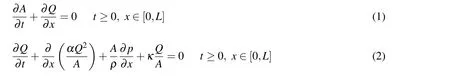
The usual method for solving this system of equations for a single compliant tube in transient and steady state flow is to use the finite element method based on the weak formulation by multiplying the mass and momentum conservation equations by weight functions and integrating over the solution domain to obtain the weak form of the system.This weak form,with suitable boundary conditions,can then be used as a basis for finite element implementation in conjunction with an iterative scheme such as Newton-Raphson method.The finite element system can also be extended to a network of interconnected deformable tubes by imposing suitable boundary conditions,based on pressure or flux constraints for instance,on all the boundary nodes,and coupling conditions on all the internal nodes.The latter conditions are normally derived from Riemann’s method of characteristics,and the conservation principles of mass and mechanical energy in the form of Bernoulli equation for inviscid flow with negligible gravitational body forces[Sochi(2013d)].More details on the finite element formulation,validation and implementation are given in[Sochi(2013a)].

The pore-scale network modeling method,which is proposed as a substitute for the finite element method in steady state flow,is established on three principles:the continuity of mass represented by the conservation of volumetric flow rate for incompressible flow,the continuity of pressure where each branching nodal point has a uniquely defined pressure value[Sochi(2013d)],and the characteristic relation for the flow of the specific fluid model in the particular structural geometry such as the flow of power law fluids in rigid tubes or the flow of Newtonian fluids in elastic ducts.The latter principle is essentially a fluid-structure interaction attribute of the adopted flow model especially in the context of compliant ducts.

In more technical terms,the pore-scale network modeling method employs an iterative scheme for solving the following matrix equation which is based on the flow continuity residual

where J is the Jacobian matrix,p is the vector of variables which represent the pressure values at the boundary and branching nodes,and r is the vector of residuals which is based on the continuity of the volumetric flow rate.For a network of interconnected tubes defined bynboundary and branching nodes the above matrix equation is defined by

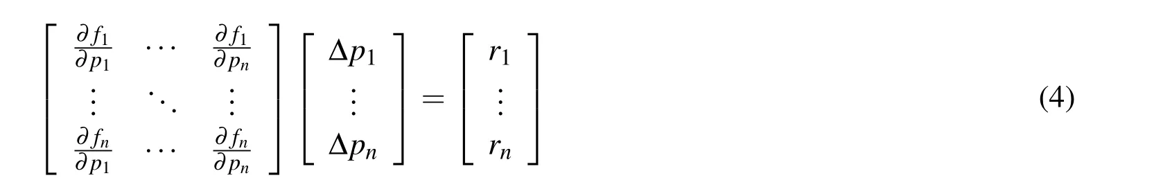
where the subscripts stand for the nodal indices,pandrare the nodal pressure and residual respectively,andfis the flow continuity residual function which,for a general nodej,is given by

In the last equation,mis the number of flow ducts connected to nodej,andQiis the volumetric flow rate in ductisigned(+/?)according to its direction with respect to the node,i.e.toward or away.For the boundary nodes,the continuity residual equations are replaced by the boundary conditions which are usually based on the pressure or flow rate constraints.In the computational implementation,the Jacobian is normally evaluated numerically by finite differencing[Sochi(2013a)].The procedure to obtain a solution by the residual-based pore-scale modeling method starts by initializing the pressure vector p with initial values.Like any other numerical technique,the rate and speed of convergence is highly dependent on the initial values of the variable vector.The system given by Equation 4 is then constructed where the Jacobian matrix and the residual vector are calculated in each iteration.The system 4 is then solved for?p,i.e.

and the vector p in iterationlis updated to obtain a new pressure vector for the next iteration(l+1),that is

This is followed by computing the norm of the residual vector from the following equation

whereris the flow continuity residual.This cycle is repeated until the norm is less than a predefined error tolerance or a certain number of iteration cycles is reached without convergence.In the last case,the operation will be deemed a failure and hence it will be aborted to be resumed possibly with improved initial values or even modified model parameters if the physical problem is flexible and allows for a certain degree of freedom.

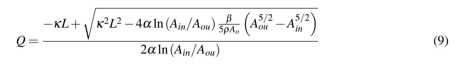
The characteristic flow relation that has to be used for computingQin the residual equation is dependent on the flow model.As for the flow of Newtonian fluids in distensible tubes based on the previously-described system of flow equations,the following analytical relation representing the one-dimensional Navier-Stokes flow in elastic tubes can be used

Other analytical or empirical or numerical relations characterizing the flow rate can also be used in this context[Sochi(2014b)].

The flow relation of Equation 9 was previously derived and validated by a one dimensional finite element method in[Sochi(2014a)].Equation 9 is based on a pressure-area constitutive elastic relation in which the pressure is proportional to the radius change with a proportionality stiffness factor that is scaled by the reference area,i.e.

In the last two equations,Aois the reference area corresponding to the reference pressure which in this equation is set to zero for convenience without affecting the generality of the results,AinandAouare the tube cross sectional area at the inlet and outlet respectively,Ais the tube cross sectional area at the actual pressure,p,as opposed to the reference pressure,andβis the tube wall stiffness coefficient which is usually defined by

wherehois the tube wall thickness at reference pressure,whileEand?are respectively the Young’s elastic modulus and Poisson’s ratio of the tube wall.

With regard to the validation of the numeric solutions obtained from the finite element and pore-scale methods,the time independent solutions of the one-dimensional finite element model can be tested for validation by satisfying the boundary and coupling conditions as well as the analytic solution given by Equation 9 on each individual duct,while the solutions of the residual-based pore-scale modeling method are validated by testing the boundary conditions and the continuity of volumetric flow rate at each internal node,as well as the analytic solution given by Equation 9 which is inevitably satisfied if the continuity equation is satisfied according to the pore-scale solution scheme.The necessity to satisfy the analytic solution on each individual tube in the finite element method is based on the fact that the flow in the individual tubes according to the underlying one-dimensional model is dependent on the imposed boundary conditions but not on the mechanism by which these conditions are imposed.In the case of finite element with tube discretization and/or employing non-linear interpolation orders,the solution at the internal points of the ducts can also be tested by satisfying the following analytical relation[Sochi(2013a)]

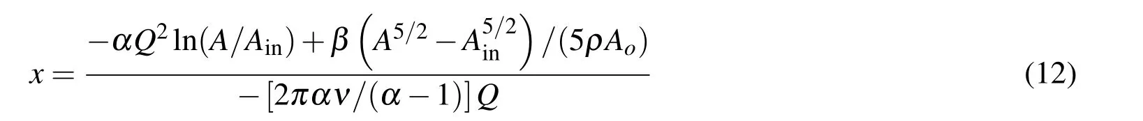
The derivation of this equation is similar to the derivation of Equation 9 but with using the inlet boundary condition only.In fact even Equation 9 can be used for testing the solution at the internal points if we assume these points as periphery nodes[Sochi(2013a)].

3 Implementation and Results

The residual-based pore-scale modeling method,as described in the last section,was implemented in a computer code with an iterative Newton-Raphson method that includes four numeric solvers(SPARSE,SUPERLU,UMFPACK,and LAPACK).The code was then tested on computer-generated networks representing distensible fluid transportation structures like ensembles of interconnected tubes or porous media.A sample of these networks are given in Figure 1.Because the residual-based pore-scale method can be used in general to obtain flow solutions for any characteristic flow that involves linear or non-linear fluid models,such as Newtonian or non-Newtonian fluids,passing through rigid or distensible networks,the code was tested first on Poiseuille and power law fluids in rigid networks[Sochi(2011b,2013b)].The results for these validation tests were exceptionally accurate with very low error margin over the whole network and with smooth convergence.We also used the one-dimensional finite element model that we briefly described in the last section for the purpose of comparison.This model was previously implemented in a computer code with a residual-based Newton-Raphson iterative solution scheme,similar to the one used in the pore-scale modeling.Full description of the finite element method,code and techniques can be found in[Sochi(2013a)].A number of pore-scale and one-dimensional finite element time independent flow simulations were carried out on our computer-generated networks using a range of physical parameters defining the fluid and structure as well as different numeric solvers with different solving schemes.Various types of pressure and flow boundary conditions were imposed in these simulations,although in most cases Dirichlettype pressure boundary conditions were applied.The finite element simulations were performed using a linear Lagrange interpolation scheme with no tube discretization to closely match the pore-scale modeling approach.All the results of the reported and unreported runs have passed the rigorous validation tests that we stated earlier in section 2.

Regarding the nature of the networks,several types of networks have been generated and used in the above-mentioned flow simulations;these include fractal,cubic and orthorhombic networks.The fractal networks are based on fractal branching patterns where each generation of the branching tubes in the network have a specific number of branches related to the number of branches in the parent generation,such as 2:1,as well as specific branching angle,radius branching ratio and length to radius ratio.The radius branching ratio is normally based on a Murray-type relation[Murray(1926a,b,c);Sochi(2013d)].The fractal networks are also characterized by the number of generations.The fractal networks used in this study have a single inlet boundary node and multiple outlet boundary nodes[Sochi(2013b)].

The cubic and orthorhombic networks are based on a cubic or orthorhombic three dimensional lattice structure where the radii of the tubes in the network can be constant or subject to statistical random distributions such as uniform distribution.These networks have a number of inlet boundary nodes on one side and a similar number of outlet boundary nodes on the opposite side while the nodes on the other four sides(i.e.the lateral)are considered internal nodes.The boundary conditions are then imposed on these inlet and outlet boundary nodes individually according to the need.A sample of the fractal,cubic and orthorhombic networks used in this investigation are shown in Figure 1.

It is noteworthy that all the networks used in the pore-scale and finite element flow simulations consist of interconnected straight cylindrical tubes where each tube is characterized by a constant radius over its entire length and spatially identified by two end nodes.These networks are totally connected,that is any node in the network can be reached from any other node by moving entirely inside the network space.As for the physical size,we used different sizes to represent different flow structures such as arterial and venous blood vascular trees and spongy porous geological media.The physical parameters used in our simulations,especially those related to the fluids and flow structures,were generally selected to represent realistic physical systems although physical parameters representing hypothetical conditions have also been used for the purpose of test and validation.However,since the current study is purely theoretical with no involvement of experimental or observational data,the validity of the reported models are not affected by the actual values of the physical parameters although this has some consequences on the speed and rate of convergence in different physical regimes.

In Figures 2 and 3 we present a sample of the above mentioned comparative simulations.In Figure 2 we plot the ratio of the flow rate obtained from the finite element model to that obtained from the pore-scale model for a fractal network with an area-preserving branching index of 2[Sochi(2013d)]where the number of tubes in each generation is twice the number in the parent generation.In these flow simulations we applied an inlet boundary pressure of 2000 Pa on the single inlet boundary node of the main branch and an outlet boundary pressure of 0.0 Pa on all the outlet boundary nodes.The results of the pore-scale and finite element models are very close although the two models differ due to the use of different branching coupling conditions,i.e.continuity of pressure for the pore-scale model and Bernoulli for the finite element.The effect of the coupling conditions on the different generations of the fractal network can be seen in Figure 2 where a generation-based con figuration is obvious.This feature is a clear indication of the effect of the coupling conditions on the deviation between the two models.

In Figure 3 we compare the pore-scale and finite element models for an inhomogeneous orthorhombic network consisting of about 11000 interconnected tubes,similar to the one depicted in Figure 1(f),where we plotted the ratio of the flow rate obtained from the two models as for the fractal network.The network is generated with a random uniform distribution for the tubes radii with a variable length in different orientations and with a variable length to radius ratio that ranges between about 5-15.The dimensions of the flow structure are 2×1.5×1 m with a constant inlet boundary pressure of 3000 Pa applied to all the nodes on the inlet side and ze-ro outlet boundary pressure applied to all the nodes on the outlet side.The fluid and structure physical parameters for the flow model are selected to roughly resemble the flow of crude oil in some elastic structure,possibly in a refinement processing plant.As seen,the pore-scale and finite element results differ significantly on most part of the network.The reason in our judgment is the effect of the branching coupling conditions(i.e.continuity of pressure and Bernoulli)which have a stronger impact in such a network than a fractal network due to the inhomogeneity with random radius distribution on one hand and the high nodal connectivity of the orthorhombic lattice on the other hand.The fluid property which significantly differs from that of the fractal network simulation may also have a role in exacerbating the discrepancy.

The results shown in these figures represent a sample of our simulations which reflect the general trend in other simulations.However the agreement between the pore-scale and finite element models is highly dependent on the flow regime and the nature of the physical problem which combines the fluid,structure and their interaction.As indicated early,the discrepancy between the two models reflects the effect of the coupling conditions,i.e.the pressure continuity for the pore-scale model and the Bernoulli condition for the finite element.The gravity of this effect is strongly dependent on the type of fluid, flow regime,inhomogeneity and connectivity.

It should be remarked that in these figures(i.e.2 and 3)we used the volumetric flow rate,rather than the nodal pressure,to make the comparison.The reason is that comparing the pressure is not possible because nodal pressure is not defined in the finite element model due to the use of the Bernoulli equation[Sochi(2013d)]where each node has a number of pressure values matching the number of the connected tubes.

4 Pore-Scale vs.Finite Element

It is difficult to make an entirely fair comparison between the pore-scale and finite element methods due mainly to the use of different coupling conditions at the branching junctions as well as different theoretical assumptions.Therefore,the pressure and flow rate fields obtained from these two methods on a given network are generally different.The difference,however,is highly dependent on the nature of the specified physical and computational conditions.

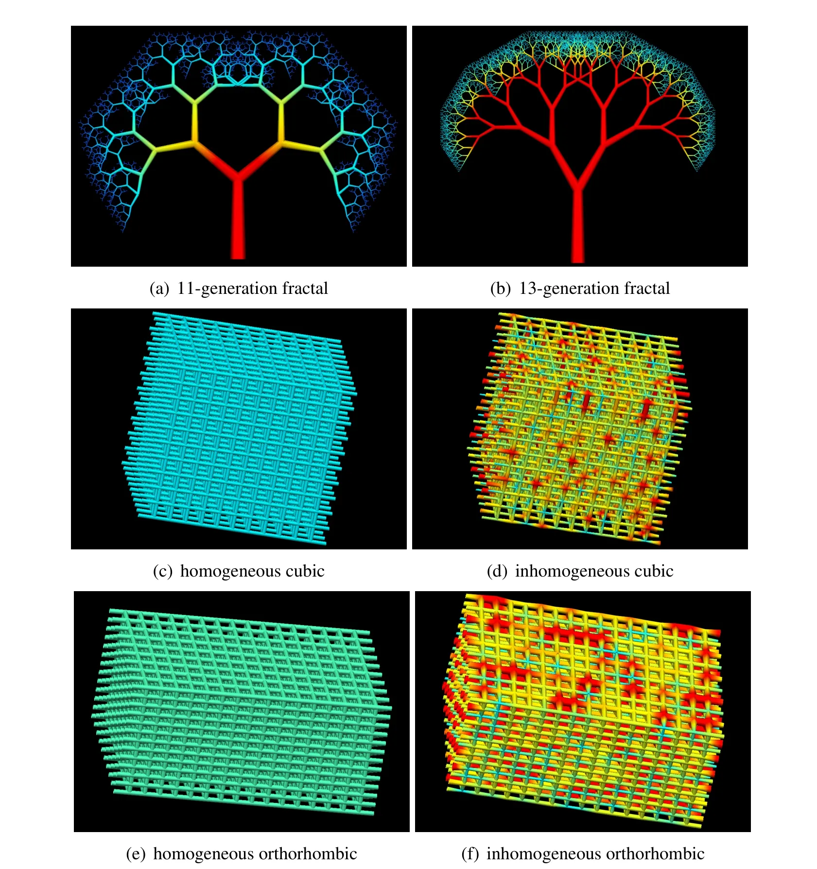
Figure 1:A sample of computer-generated fractal,cubic and orthorhombic networks used in the current investigation.

One of the advantages of the pore-scale modeling method over the finite element method,in addition to the general advantages of the pore-scale modeling approach which were outlined earlier,is that when pore-scale method converges it usually converges to the underlying analytic solution with negligible marginal errors over the whole network,while the finite element method normally converges with significant errors over some of the network ducts especially those with eccentric geometric characteristics such as very low length to radius ratio[Sochi(2013a)].It may also be argued that the coupling condition used in the pore-scale modeling method,which is based on the continuity of pressure,is better than the corresponding coupling condition used in the finite element method which is based on the Bernoulli inviscid flow with discontinuous pressure at the nodal points.Some of the criticism to the use of Bernoulli as a coupling condition is outlined in[Sochi(2013d)].Another advantage of the pore-scale modeling is that it is generally more stable than the finite element with a better convergence behavior due partly to the simpler pore-scale computational infrastructure.

The main advantage of the finite element method over the pore-scale modeling method is that it accommodates time dependent flow naturally,as well as time independent flow,while pore-scale modeling in its current formulation is capable only of dealing with time independent flow.Moreover,the finite element method may be better suited for describing other one-dimensional transportation phenomena such as wave propagation and reflection in deformable networks.However,time dependent flow can be simulated within the pore-scale modeling framework as a series of time independent frames although this is not really a time dependent flow but rather a pseudo time dependent.Another advantage of the finite element method is that it is capable,through the use of segment discretization and higher orders of interpolation,of computing the pressure and flow rate fields at the internal points along the tubes length and not only on the tubes periphery points at the nodal junctions.However,due to the incompressibility of the flow,computing the flow rate at the internal points is redundant as it is identical to the flow rate at the end points.With regard to computing the pressure field on the internal points,it can also be obtained by pore-scale modeling method through the application of Equation 12 to the solution obtained on the individual ducts.Moreover,it can be obtained by creating internal nodal junctions along the tubes through the use of tube discretization,similar to the discretization in the finite element method.

With regard to the size of the problem,which directly influences the ensuing memory cost as well as the CPU time,the number of degrees of freedom for the pore-scale model is half the number of degrees of freedom for the one-dimensional finite element model due to the fact that the former has one variable only(p)while the latter has two variables(pandQ).This estimation of the finite element computational cost is based on using a linear interpolation scheme with no tube discretization;and hence this cost will substantially increase with the use of discretization and/or higher orders of interpolation.The computational cost for both models also depends on the type of the solver used such as being sparse or dense,and direct or iterative,as well as some problem-specific implementation overheads.

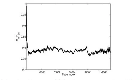
Figure 3:The ratio of flow rate of finite element to pore-scale models versus tube index for an inhomogeneous orthorhombic network.The network consists of about 11000 tubes with different lengths and length to radius ratios as explained in the main text.The parameters for these simulations are:β=236.3 Pa.m,ρ =860.0 kg.m?3,μ =0.075 Pa.s,and α =1.2.The inlet and outlet pressures are:pi=3000 Pa and po=0.0 Pa.The fluid and structure parameters are chosen to approximately match the transport of crude oil through an elastic structure.

CPU processing time depends on several factors such as the size and type of the network,the initial values for the flow solutions,the parameters of the fluid and tubes,the employed numerical solver,and the assumed pressure-area constitutive relation.Typical processing time for a single run of the pore-scale network model on a typical laptop or desktop computer ranges between a few seconds to few minutes using a single processor with an average speed of 2-3 gigahertz.The CPU processing time for the time independent finite element model is comparable to the processing time of the pore-scale network model.In both cases,the final convergence in a typical problem is normally reached within 3-7 Newton-Raphson iterations depending mainly on the initial values.

5 Convergence Issues

Like the one-dimensional Navier-Stokes finite element model,the residual-based pore-scale method may suffer from convergence difficulties due to the highly nonlinear nature of the flow model.The nonlinearity increases,and hence the convergence difficulties aggravate,with increasing the pressure gradient across the flow domain.The nonlinearity also increases with eccentric values representing the fluid and structure parameters such as the fluid viscosity or wall distensibility.Several numerical tricks and stabilization techniques can be used to improve the rate and speed of convergence.These include non-dimensionalization of the flow equations,using a variety of unit systems such as m.kg.s or mm.g.s or m.g.s for the input data and parameters,and scaling the network flow model up or down to obtain a similarity solution that can be scaled back to obtain the final solution.The error tolerance for the convergence criterion which is based on the residual norm may also be increased to enhance the rate and speed of convergence.Despite the fact that the use of relatively large error tolerance can cause a convergence to a wrong solution or to a solution with large errors,the solution can always be tested by the above-mentioned validation metrics and hence it is accepted or rejected according to the adopted approval criteria[Sochi(2013a)].

Other convergence-enhancing methods can also be used.In the highly non-linear cases,the initial values to initiate the variable vector can be obtained from a Poiseuille solution which can be easily acquired within the same code.The convergence,as indicated already,becomes more difficult with increasing the pressure gradient across the flow domain,due to an increase in the nonlinearity.An effective approach to obtain a solution in such cases is to step up through a pressure ladder by gradual increase in the pressure gradient where the solution obtained from one step is used as an initial value for the next step.Although this usually increases the computational cost,the increase in most cases is not substantial because the convergence becomes rapid with the use of good initial values that are close to the solution.The convergence rate and speed may also be improved by adjusting the flow parameters.Although the parameters are dependent on the nature of the physical problem and hence they are not a matter of choice,there may be some freedom in tuning some non-critical parameters.In particular,adjusting the correction factor for the axial momentum flux,α,can improve the convergence and quality of solution.The rate and speed of convergence may also depend on the employed numerical solver.

Another possible convergence trick is to use a large error margin for the residual norm to obtain an approximate solution which can be used as an initial guess for a second run with a smaller error margin.On repeating this process,with progressively reducing the error margin,a reasonably accurate solution can be obtained eventually.It should be remarked that the pore-scale and finite element models have generally different convergence behaviors where each converges better than the other for certain flow regimes or fluid-structure physical problems.However,in general the pore-scale model has a better convergence behavior with a smaller error,as indicated earlier.These issues,however,are strongly dependent on the implementation and practical coding aspects.

6 Conclusions

In this paper,a pore-scale modeling method has been proposed and used to obtain the pressure and flow fields in distensible networks and porous media.This method is based on a residual formulation obtained from the continuity of volumetric flow rate at the branching junctions with a Newton-Raphson iterative numeric technique for solving a system of simultaneous non-linear equations.An analytical relation linking the flow rate in distensible tubes to the boundary pressures is exploited in this formulation.This flow relation is based on a pressure-area constitutive equation derived from elastic tube deformability characteristics.

A comparison between the proposed pore-scale network modeling approach and the traditional one-dimensional Navier-Stokes finite element approach has also been conducted with a main conclusion that pore-scale modeling method has obvious practical and theoretical advantages,although it suffers from some limitations related mainly to its static time independent nature.We therefore believe that although the pore-scale modeling approach cannot totally replace the traditional methods for obtaining the flow rate and pressure fields over networks of interconnected deformable ducts,it is a valuable addition to the tools used in such flow simulation studies.

Ambrosi,D.(2002): Infiltration through Deformable Porous Media.ZAMM Journal of Applied Mathematics and Mechanics,vol.82,no.2,pp.115–124.

Barnard,A.C.L.;Hunt,W.A.;Timlake,W.P.;Varley,E.(1966):A Theory of Fluid Flow in Compliant Tubes.Biophysical Journal,vol.6,no.6,pp.717–724.

Chapelle,D.;Gerbeau,J.F.;Sainte-Marie,J.;Vignon-Clementel,I.E.(2010):A poroelastic model valid in large strains with applications to perfusion in cardiac modeling.Computational Mechanics,vol.46,no.1,pp.91–101.

Chen,H.;Ewing,R.E.;Lyons,S.L.;Qin,G.;Sun,T.;Yale,D.P.(2000):A Numerical Algorithm for Single Phase Fluid Flow in Elastic Porous Media.Lecture Notes in Physics-Numerical Treatment of Multiphase Flows in Porous Media,vol.552,pp.80–92.

Coussy,O.(2004):Poromechanics.John Wiley&Sons Ltd,1st edition.

Coussy,O.(2010):Mechanics and Physics of Porous Solids.John Wiley&Sons Ltd,1st edition.

Formaggia,L.;Lamponi,D.;Quarteroni,A.(2003):One-dimensional models for blood flow in arteries.Journal of Engineering Mathematics,vol.47,no.3/4,pp.251–276.

Huyghe,J.M.;Arts,T.;van Campen,D.H.;Reneman,R.S.(1992):Porous medium finite element model of the beating left ventricle.American Journal of Physiology-Heart and Circulatory Physiology,vol.262,no.4,pp.H1256–H1267.

Ju,B.;Wu,Y.;Fan,T.(2011): Study on fluid flow in nonlinear elastic porous media:Experimental and modeling approaches.Journal of Petroleum Science and Engineering,vol.76,no.3-4,pp.205–211.

Klubertanz,G.;Bouchelaghem,F.;Laloui,L.;Vulliet,L.(2003): Miscible and immiscible multiphase flow in deformable porous media.Mathematical and Computer Modelling,vol.37,no.5-6,pp.571–582.

Krenz,G.S.;Dawson,C.A.(2003):Flow and pressure distributions in vascular networks consisting of distensible vessels.American Journal of Physiology-Heart and Circulatory Physiology,vol.284,no.6,pp.H2192–H2203.

Mabotuwana,T.D.S.;Cheng,L.K.;Pullan,A.J.(2007):A model of blood flow in the mesenteric arterial system.BioMedical Engineering On Line,vol.6,pp.17.lf ow in deformable arteries by 3D and 1D models.Mathematical and Computer Modelling,vol.49,no.11-12,pp.2152–2160.

Sochi,T.(2007):Pore-Scale Modeling of Non-Newtonian Flow in Porous Media.PhD thesis,Imperial College London.

Sochi,T.(2009):Pore-scale modeling of viscoelastic flow in porous media using a Bautista-Manero fluid.International Journal of Heat and Fluid Flow,vol.30,no.6,pp.1202–1217.

Sochi,T.(2010a): Modelling the Flow of Yield-Stress Fluids in Porous Media.Transport in Porous Media,vol.85,no.2,pp.489–503.

Sochi,T.(2010b):Non-Newtonian Flow in Porous Media.Polymer,vol.51,no.22,pp.5007–5023.

Sochi,T.(2010c):Computational Techniques for Modeling Non-Newtonian Flow in Porous Media.International Journal of Modeling,Simulation,and Scientific Computing,vol.1,no.2,pp.239–256.

Sochi,T.(2010d):Flow of Non-Newtonian Fluids in Porous Media.Journal of Polymer Science Part B,vol.48,no.23,pp.2437–2467.

Sochi,T.(2011a):Slip at Fluid-Solid Interface.Polymer Reviews,vol.51,no.4,pp.309–340.

Sochi,T.(2011b):The flow of power-law fluids in axisymmetric corrugated tubes.Journal of Petroleum Science and Engineering,vol.78,no.3-4,pp.582–585.

Sochi,T.(2013a):One-Dimensional Navier-Stokes Finite Element Flow Model.arXiv:1304.2320,Technical Report.

Sochi,T.(2013b): Comparing Poiseuille with 1D Navier-Stokes Flow in Rigid and Distensible Tubes and Networks.arXiv:1305.2546,Submitted.

Murray,C.D.(1926a): The Physiological Principle of Minimum Work I.The Vascular System and the Cost of Blood Volume.Proceedings of the National A-cademy of Sciences of the United States of America,vol.12,no.3,pp.207–214.

Murray,C.D.(1926b): The Physiological Principle of Minimum Work.II.Oxygen Exchange in Capillaries.Proceedings of the National Academy of Sciences of the United States of America,vol.12,no.5,pp.299–304.

Murray,C.D.(1926c):The physiological principle of minimum work applied to the angle of branching of arteries.The Journal of General Physiology,vol.9,no.6,pp.835–841.

Nobile,F.(2009): Coupling strategies for the numerical simulation of blood

Sochi,T.(2013c):Newtonian Flow in Converging-Diverging Capillaries.International Journal of Modeling,Simulation,and Scientific Computing,vol.04,no.03,pp.1350011.

Sochi,T.(2013d):Fluid Flow at Branching Junctions.arXiv:1309.0227,Submitted.

Sochi,T.(2014a): Navier-Stokes Flow in Cylindrical Elastic Tubes.Journal of Applied Fluid Mechanics,Accepted.

Sochi,T.(2014b):Using the Euler-Lagrange variational principle to obtain flow relations for generalized Newtonian fluids.Rheologica Acta,vol.53,no.1,pp.15–22.

Sorbie,K.S.;Clifford,P.J.;Jones,E.R.W.(1989):The Rheology of Pseudoplastic Fluids in Porous Media Using Network Modeling.Journal of Colloid and Interface Science,vol.130,no.2,pp.508–534.

Sorbie,K.S.(1990): Depleted layer effects in polymer flow through porous media:II.Network calculations.Journal of Colloid and Interface Science,vol.139,no.2,pp.315–323.

Sorbie,K.S.(1991):Polymer-Improved Oil Recovery.Blackie and Son Ltd.

Spiegelman,M.(1993): Flow in deformable porous media I:Simple Analysis.Journal of Fluid Mechanics,vol.247,pp.17–38.

Valvatne,P.H.(2004):Predictive pore-scale modelling of multiphase flow.PhD thesis,Imperial College London.

Whitaker,S.(1986):Flow in porous media III:Deformable media.Transport in Porous Media,vol.1,no.2,pp.127–154.