Comparison of smoothness-constrained and geostatistically based cross-borehole electrical resistivity tomography for characterization of solute tracer plumes

Comparison of smoothness-constrained and geostatistically based cross-borehole electrical resistivity tomography for characterization of solute tracer plumes

Experiments using electrical resistivity tomography(ERT)have shown promising results in reducing the uncertainty of solute plume characteristics related to estimates based on the analysis of local point measurements only.To explore the similarities and differences between two cross-borehole ERT inversion approaches for characterizing salttracer plumes,namely the classicalsmoothness-constrained inversion and a geostatistically based approach,we performed two-dimensional synthetic experiments.Simplifying assumptions about the solute transport modeland the electricalforward and inverse modelallowed us to study the sensitivity of the ERT inversion approaches towards a variety of basic conditions,including the numberofboreholes,measurementschemes,contrastbetween the plume and background electricalconductivity,use of a priori knowledge,and point conditioning.The results show that geostatistically based and smoothness-constrained inversions of electrical resistance data yield plume characteristics of similar quality,which can be further improved when point measurements are incorporated and advantageous measurement schemes are chosen.As expected,an increased number of boreholes included in the ERT measurement layout can highly improve the quality of inferred plume characteristics,while in this case the benefits of pointconditioning and advantageous measurement schemes diminish.Both ERT inversion approaches are similarly sensitive to the noise levelof the data and the contrastbetween the solute plume and background electricalconductivity,and robustwith regard to biased inputparameters,such as mean concentration,variance,and correlation length of the plume.Although sophisticated inversion schemes have recently become available,in which fl ow and transport as well as electrical forward models are coupled,these schemes effectively rely on a relatively simple geometrical parameterization of the hydrogeological model. Therefore,we believe that standard uncoupled ERT inverse approaches,like the ones discussed and assessed in this paper,will continue to be important to the imaging and characterization of solute plumes in many real-world applications.

Electrical resistivity tomography;Inversion technique;Solute tracer plume;Synthetic experiment;Plume characteristics

1.Introduction

Subsurface heterogeneity has a significant effect on various subsurface flow and transport processes.A finite number of local measurements in boreholes can only provide limitedinformation about subsurface heterogeneity and thus can lead to uncertain process prediction.For example,characterization of transport processes based solely on local concentration measurements from groundwater observation wells or multilevel samplers is difficult,even if the spatial sampling density is high(Mackay et al.,1986;LeBlanc et al.,1991;Boggs et al.,1992;Vereecken et al.,2000).However,synthetic, laboratory,and fi eld experiments have yielded promising results helpful to overcoming these limitations by incorporating geophysical tomographic data in the delineation of salt tracer plumes(Rubin and Hubbard,2005;Vereecken et al.,2006; Binley et al.,2015).In particular,studies have shown that time-lapse electricalresistivity tomography(ERT)is a suitable tool for characterizing water saturation(Ganz et al.,2015; Chou et al.,2016)and transport processes at various scales (Kemna et al.,2006;Revil et al.,2012;Singha et al.,2015). Binley etal.(1996),Koesteletal.(2009a,b),and Persson etal. (2015),amongst others,have shown the benefit of ERT in the course of laboratory-scale solute tracer experiments.At the scale of tank experiments,Daily et al.(1995)and Slater et al. (2002),and at the field scale,Kemna et al.(2002),Singha and Gorelick(2005),Looms et al.(2008),Nguyen et al.(2009), Mu¨ller et al.(2010),and Haarder et al.(2015)have demonstrated the advantage of ERT to imaging and characterization of transport processes.These studies utilized a standard regularization approach in the ERT inversion with a smoothness constraint to overcome the inherent ill-posedness of the inverse problem.However,ERT inversion schemes with a geostatistically based constraint have also been proposed(Linde et al.,2006;Hermans et al.,2012)and found to be superior to deterministic approaches such as the smoothnessconstrained inversion if local point measurements of the soughtparameter distribution are used to condition the inverse solution(Hermans et al.,2012,2016).

In subsurface hydrology,inverse problems are well known, starting from classical pumping test analysis.Here,homogeneity in the hydraulic conductivity is assumed and,therefore, the inverse problem can be solved using an analyticalsolution. To overcome the assumption of homogeneity,hydraulic tomography,which represents a hydraulic analog of ERT,has been developed(Butler and Liu,1993;Gottlieb and Dietrich, 1995;Illman et al.,2015).While a smoothness-constrained regularization approach is commonly used in ERT,the groundwater flow inverse problem is often solved using geostatistical approaches(Zimmerman et al.,1998).In particular, the hydraulic tomography inverse problem has been solved by Yeh and Liu(2000),Wu etal.(2005),and Zhu and Yeh(2005) using geostatistical approaches.Due to the similarity between water flow and electric currentflow in saturated porous media, the corresponding forward and inverse problems for the two processes are similar.Yeh et al.(2002)developed an inverse approach,the sequentialsuccessive linear estimator(SSLE),to deal with electrical resistivity data based on the geostatistical inverse approach developed for hydraulic tomography(Yeh and Liu,2000).

Although many studies have shown the potential of ERT in better characterization of flow and transportin the subsurface, there are a couple of challenges associated with ERT.Importantly,electric currentflow in the subsurface is governed by two different mechanisms:electrolytic conduction in the pore fluid and surface conduction along mineral-fluid interfaces.The imaging of a solute saltplume facilitates primarily electrolytic conduction,butsurface conduction affects the relationship between measured bulk conductivity and solute concentration. Therefore,ifthe subsurface is notwelldescribed in terms ofthe spatial distribution of material characteristics contributing to the different conduction mechanisms(e.g.,clay content),in generalthe signalof interestcannotbe extracted(Kemna etal., 2002).This diffi culty,however,is less critical in ERT monitoring surveys of solute transport where observed changes are preliminary due to the changes in electrolytic conductivity associated with salinity variations,particularly when difference-inversion schemes are applied(LaBrecque and Yang,2000;Kemna et al.,2002).Although connected to extensive coring,the petrophysicalrelationships,here the bulk electrical conductivity as a function of the solute salt concentration,can be determined in laboratory experiments at the column scale.However,since these petrophysicalrelationships are generally determined ata scale beyond the spatialresolution of field-scale ERT,the quality of fi eld-scale inversion results based on such relationships is dependent on the correct upscaling of the relationships from the laboratory scale to the field scale(Moysey et al.,2005).

Smoothness-constrained ERT inversion procedures are potentially inappropriate if signifi cant spatial variations are present in the subsurface,which may result from the heterogeneous nature of a tracer plume in a heterogeneous aquifer. Accordingly,Kemna et al.(2002),Vanderborght et al.(2005), Day-Lewis et al.(2005),Pidlisecky et al.(2011),and Korteland and Heimovaara(2015)have found that transport properties inferred from smoothness-constrained ERT results are sensitive to the amount of smoothing imposed by the inversion procedure.This in turn can lead to biased spatial moments of the plume,including an underestimation of the zeroth moment and an overestimation of the second centered spatial moment(Vanderborght et al.,2005;Day-Lewis et al., 2007).We further recognize that,while a solute plume in a heterogeneous aquifer can be highly irregular,it can be characterized in a geostatistical sense,for example in terms of its mean position,lateral spreading,and spatial correlation structure.If the heterogeneity of the hydraulic conductivity distribution is welldetermined at a site,the existing stochastic theories of solute transport processes can estimate plume statistics based on the statistics of the hydraulic conductivity field(Vanderborght,2001).These plume statistics can serve as a priori knowledge about the plume.Therefore,we hypothesized thata geostatistically based ERT inversion approach,the SSLE in this study,incorporating a priori knowledge of the geostatistical characteristics of a plume and optionally in addition some direct point measurements of the plume concentration,can lead to an improved image of the subsurface electrical conductivity distribution associated with the plume.

The work presented here aims at providing a better understanding of the suitability,similarities,and differences ofthe two ERT inversion approaches outlined above,i.e.,a classical smoothness-constrained inversion and a geostatistically based approach.This work is based on synthetic,crossborehole ERT experiments,in order to image a synthetic solute saltplume.For the sake of simplicity,itis assumed that,based on a homogeneous background bulk conductivity distribution, solute concentration is linearly related to bulk electrical conductivity changes.Transportmodeling and ERT simulation are performed two-dimensionally,which is considered sufficient for providing qualitative insight into the targeted issues addressed here.We examined the effects on the quality of the estimated electrical conductivity distribution using the different ERT inversion procedures for different sets of statistical and deterministic(point conditioning)a priori knowledge,amount of noise in the measurement data,and concentration contrast between solute plume and background electrical conductivity.As it is well known that ERT measurement schemes and electrode layout have a strong impact on the quality of ERT inversion results(Loke et al.,2015),we also included two different cross-borehole measurement schemes and three different electrode layouts.

The paper is organized in the following manner:First,the two approaches for electrical inverse modeling are outlined. Then,the layout of the synthetic experiments is presented. Finally,an integrated analysis of the results of the ERT inversions based on the two approaches is provided.

2.Electrical inverse modeling

The imaging of electrical conductivity(σb)in the subsurface by ERT is based on the inversion of a set of resistance measurements,i.e.,the ratios of measured voltage to injected current strength,on a given array of electrodes.Given the nonlinearity of the underlying forward problem,i.e.,the solution of the Poisson equation,electrical inversion schemes proceed in iterations through modeling runs looping forward, comparing predicted and measured data,and updating the estimate of the electrical resistivity distribution with a view to reducing data misfit.This section outlines the principles of the smoothness-constrained inversion and the SSLE approaches, as implemented in this work,to accomplish the iterative inversion.

2.1.Smoothness-constrained inversion

Smoothness-constrained inversion is based on the idea of searching for the model with the simplest structure,i.e.,the smoothest model,which is used to fit the measurements.This is accomplished by solving an optimization problem in which the roughness of the model is minimized subject to fi tting the data to a pre-defined degree(Constable et al.,1987; LaBrecque et al.,1996;Koestel et al.,2008).

In this study,the finite element-based two-dimensional smoothness-constrained inversion scheme proposed by Kemna (2000)was used.The log resistances were used as data and log conductivities of the fi nite elements as model parameters.The objective function that is minimized by means of a series of Gauss-Newton type inverse steps comprises the L2norm(the least squared deviation)of the error-weighted data misfit and the L2norm of the first-order model roughness,with both terms being balanced by a regularization parameter.At each iteration step,a univariate search was performed(deGroot-Hedlin and Constable,1990)to find the maximum value of the regularization parameter(implying the smoothest model), which locally minimizes the data misfi t or,in the fi nal iteration,yields the data misfit target value according to the error present in the data.

In this study,the data errors were assumed to be Gaussian and uncorrelated,which results in a diagonal data weighting matrix in the data misfi t term containing the inverse standard deviations of the data in diagonal entries(we note that a relative Gaussian resistance error of 5%,for example,corresponds to a standard deviation of the log resistance datum of 0.05 due to the involved log transformation).

Optionally,the weighting of model roughness in the horizontal and vertical directions,respectively,can be adjusted separately in the objective function through two additional smoothing parameters,the horizontal and vertical smoothing parameters(Ellis and Oldenburg,1994;Kemna et al.,2002), and the ratio of the two parameters defi nes an anisotropy of smoothing.Importantly,this smoothing anisotropy ratio corresponds directly to the ratio of the horizontal to vertical correlation lengths of the a priorimodelcovariance function as assumed in a geostatistical inverse formulation(Kitanidis, 1999).More details on the inversion algorithm,as well as the solution of the underlying forward problem,can be found in Kemna(2000).

2.2.Sequential successive linear estimator(SSLE)

The SSLE is a geostatistical inverse approach that conceptualizes the parameter fi eld as a stochastic process in space. Given available observed ERT data,the estimated parameter fi eld approximates the conditional mean of the stochastic process,based on the spatial structure and spatial crosscorrelation of the parameter and process fi elds.Using this conditional stochastic concept,the SSLE addresses uncertainty of the estimates due to both spatial variability and errors in measurements.Detailed description of the SSLE for groundwater hydrological applications is available in Yeh and Liu(2000)and for ERT applications in Yeh et al.(2002),Liu and Yeh(2004),and Yeh et al.(2006).

Briefl y,the SSLE treats log electrical conductivity as a primary variable and voltage as a secondary variable(in this study a unity current strength was assumed).The SSLE starts with the classic cokriging method using direct measurements of the primary variable and measurements of the secondary variable to obtain the first estimate of the primary variable:

whereχ*and v*are nχ*×1 and nv*×1 vectors of measured primary and secondary variables,respectively,andαandβare m×nχ*and m×nv*vectors of weights associated with themeasurements(m is the total number of primary variables to be estimated in a domain).The weights are calculated based on spatial moments(means and covariances)of the primary variable,the spatial covariances of secondary variables,and spatial cross-covariances between primary and secondary variables.These covariances are determined by fi rst-order approximations.

Cokriging is a linear estimator.To consider the nonlinear relation between the electrical conductivity and voltages,a linear estimator is used iteratively and this approach is called the successive linear estimator(SLE)technique.This technique uses the fi rst estimates of the primary variable as inputs into the forward modelto approximate the conditionalmean of the secondary variables.The differences between calculated and observed secondary variables(v*and vr,respectively, where the superscript r is the iteration index)are subsequently used in conjunction with associated weights,ωr,to improve the estimate,χr+1,iteratively.That is,

Similar to cokriging,these weights in SLE represent contributions of the differences to the estimate ata given location. These weights are obtained by solving a system of equations that involve conditional covariances and cross-covariances, which are derived from the previous iteration.After improved estimates are obtained,the conditional covariance,is updated using a fi rst-order approximation:

The secondary information collected from each ERT survey is added into the inverse process sequentially.This approach is then called SSLE.The SSLE uses a loop iteration scheme to sequentially incorporate the different current injections and corresponding voltage(resistance)measurements given in the ERT data set(see Zhu and Yeh(2005)for the hydraulic inverse problem).To account for equal weighting of each current injection in the present study,we fi xed the number of iterations per injection.The SLE is similar to the Kalman fi lter,but the Kalman fi lter updates the estimate and covariances when new measurements at new time steps become available(Hao et al.,2008).

3.Synthetic experiments

In section 3.1 we present the generation of a synthetic twodimensional solute plume,based on flow and transport modeling.We further present the transformation of the twodimensional concentration field(salt plume)into a corresponding two-dimensional electrical conductivity fi eld.These two-dimensionalfi elds serve as the true solute tracerplume and its corresponding electrical conductivity field,respectively.In section 3.2 we present the procedures and layouts of synthetic cross-borehole ERT surveys to map the true salt plume.Our primary objective was to compare different inversion methods. Although our synthetic example was designed to represent a realistic case,we made some simplifying assumptions in order to speed up the modelinversion(a two-dimensional simulation domain without density-driven flow).These simplifications should not influence the comparison of the two inversion methods.

3.1.Flow and transport modeling

The firststep of the synthetic experimentwas the generation of a single realization of a heterogeneous and statistically anisotropic hydraulic conductivity fi eld(Fig.1).In Fig.1, Y=ln K,where K is the hydraulic conductivity(m/s).Using a Kraichnan generator(Kraichnan,1970),a two-dimensional hydraulic conductivity field with a length(x)of 30 m and a height(y)of5 m was generated.The grid size was 0.5 m in the x direction and 0.25 m in the y direction,resulting in a 1200-element grid.The geometric mean of the hydraulic conductivity was 2.89×10-3m/s and the variance ofthe log-transformed hydraulic conductivity was 1.Choosing an exponentialmodel, the correlation length was 5 m in the horizontal direction and 1 m in the vertical direction.A constant porosity of 0.25 was assumed for the entire modeling domain.

In the second step,we used the generated hydraulic conductivity field to solve the fl ow equation numerically with the finite-element code TRACE(Vereecken et al.,1994,1996). The left and right boundaries of the field were assigned as constant head boundaries resulting in a mean hydraulic gradient of 0.001 from left to right.The top and bottom boundaries were assigned as no fl ux boundary conditions.The resulting fl ow fi eld shows a mean fl ow direction from left to right.

In the third step,the calculated fl ow fi eld was used to simulate transport of a non-reactive salt tracer after injection, which was parallel to the vertical axis,4.75 m from the left boundary(Fig.1).An open borehole tracer injection was simulated.The transport modeling was carried out using the particle tracking code PARTRACE (Seidemann,1996; Neuendorf,1996;Vereecken et al.,1996).With this procedure 2 million particles were injected,and the local dispersivity was set to 0.1 m in the longitudinaldirection and 0.01 m in the transversal direction.The transport modeling resulted in twodimensional concentration fi elds for every time step of the modeling procedure.For the synthetic ERT study,we chose the concentration distribution eight days after injection and used it as the true concentration field,which was then equipped with synthetic boreholes for ERT,implying that the general location of the plume is known a priori.

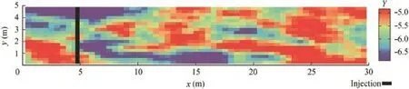
Fig.1.Log hydraulic conductivity field and location of tracer injection.

Assuming that tortuosity,porosity,and electrical surface conduction are space-invariant,and the electrical surface conduction is concentration-independent,the relationship between bulk electrical conductivity and salt concentration becomes linear and space-invariant(Nguyen et al.,2009). Based on these assumptions,we converted the simulated concentration distribution after a transport time of eight days into an electrical conductivity distribution based on the linear relationshipσb=0.01+0.18C,where C is the dimensionless concentration.This led to an electrical conductivity distribution with a maximum value of 0.1 S/m and a background electrical conductivity value of 0.01 S/m(Fig.2(a)).Subsequent synthetic ERT experiments were conducted for this twodimensional electrical conductivity distribution.Based on this distribution we also determined our a priori knowledge,i.e., the mean and the variance of the log-transformed electrical conductivity distribution with the values of 0.014 S/m and 0.31,respectively,the horizontal and vertical correlation lengths with the values of 2.36 m and 0.56 m,respectively,and the point measurements of the distribution.The a priori knowledge can be used to condition the inverse procedure.

The described electrical conductivity distribution exhibits a maximum contrast of 10 between the salt plume and the background.To study the influence of the contrast we generated synthetically modified electrical conductivity distributions using a linear relationship:

whereσmodis the modifi ed electrical conductivity,σbgis the background electrical conductivity,σdesis the described electrical conductivity,and N is a factor defining the contrast of the modifi ed electrical conductivity distribution.In our synthetic experiment,we set N to be 0.1,0.2,0.5,2,and 5. This results in five additional true electrical conductivity fields,with their maximum contrasts between the salt plume and the background ranging from 1.9 to 46.

As presented,the generation of the electrical conductivity fields is the result of fl ow and transport modeling,which neglects density effects.This is nota very realistic assumption in terms of transport of salt plumes,which can be crucially infl uenced by density-driven flow.However,the previously generated electrical conductivity fi elds allow for an integrated analysis of ERT for electrical conductivity fields of the same shape,but different values of contrast between plume and background.

3.2.Electrical modeling

We conducted ERT surveys with three different electrode layouts:(1)three vertical boreholes at positions 5 m,15 m, and 25 m away from the left-hand boundary(Fig.2(b));(2) fi ve boreholes at positions 5 m,10 m,15 m,20 m,and 25 m away from the same boundary(Fig.2(d));and(3)nine boreholes at positions 5 m,7.5 m,10 m,12.5 m,15 m,17.5 m, 20 m,22.5 m,and 25 m away from the boundary(Fig.2(f)). Along each of these boreholes ten electrodes with a separation distance of 0.5 m were assumed.These electrodes were used for current injection and electric voltage measurements.

The forward modeling subroutines in the SSLE(Yeh et al., 2002)and the smoothness-constrained regularization approach (Kemna,2000)were used to calculate the electric potential fi elds caused by current injection at selected locations of the generated electrical conductivity distribution.

In principle,all possible pairs of electrodes could be used for current injection and electric voltage measurement,and with more measurements the resultwill be better.However,in practice,one has to compromise between the number of measurements performed and the time of the ERT survey as well as the duration of the processing of the ERT measurements.In this study,we used two different types of injection and measurement schemes:a regular skip-one dipole-dipole measurementscheme(hereafter simply referred to as skip-one scheme),which is a common layout for cross-borehole ERT (Kemna et al.,2002),and,alternatively,a dipole-dipole measurement scheme with cross-borehole current injection(hereafter simply referred to as cross-borehole scheme).The skipone measurement scheme consisted of current injection dipoles and measurement dipoles with electrodes at an interval of 1 m in the vertical direction,respectively.This scheme led to 24,40,and 72 current injections for the three-,fi ve-,and nine-borehole layouts,respectively.In the same manner,the voltage measurements were undertaken at measurement dipoles in the borehole where current was injected and in the neighboring boreholes.The cross-borehole measurement scheme consisted of current injection dipoles with electrodes located in neighboring boreholes.The depth of the electrode position was identical in the two boreholes.Thus,ten current injections were performed in a pair of neighboring boreholes. This scheme led to 20,40,and 80 current injections for the three-,five-,and nine-borehole layouts,respectively.Other than the current injection electrodes,the electrodes of the measurementdipoles were located in the same borehole with a dipole length of 0.5 m in the vertical direction.

The quality of an ERT inversion result is strongly dependent on the measurement error.To test the effect of data noise in the present study,5%-20%noise was added to the synthetic ERT voltage measurements.The added noise was lognormally distributed,uncorrelated,and unbiased.

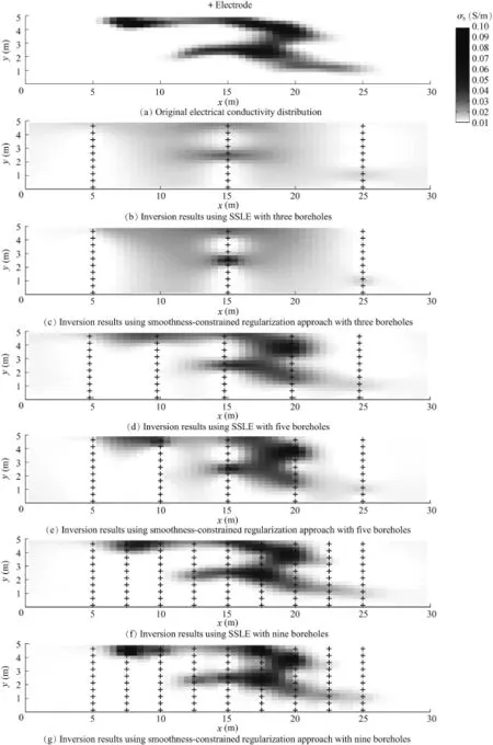
Fig.2.Originalelectricalconductivity distribution and inversion results for cross-borehole measurement scheme based on measurement data at 5%noise level.

The synthetic data sets,including different noise levels, were used as inputs to the two inverse modeling procedures. For the SSLE approach and the smoothness-constrained inversion approach,we used the same boundary conditions as in the forward model.There were no fl ux boundaries on the right,left,and top boundaries,and constant potential at the bottom.In addition to the inversion runs without any conditioning,electrical conductivity values at six different depths ata distance of 20 m in the horizontaldirection were assumed to be known and used in the SSLE to condition the inverse procedure(Fig.3).These known electrical conductivity values simulate local in situ measurements of electrical conductivity as they can be obtained from multi-level groundwater sampling.In Fig.3,the conditioning points are shown together with SSLE inversion results including estimation variances (σ2)of the log-transformed electrical conductivity.

4.Results and discussion

The results of the synthetic studies are visualized and analyzed in terms of statistics and spatial moments of the salt plume(Delleur,1999).Although the images show the entire electrical conductivity distribution,statistics and spatial moments focus on the area between boreholes,i.e.,between 5 m and 25 m along the length axis.

4.1.Number of boreholes

In Fig.2 the electrical conductivity distribution of the true salt plume is shown together with inverted electrical conductivity distributions of the salt plume,based on noisy measurement data(at 5%noise level).As expected,with an increasing number of boreholes,the results of the inversions are improved.This holds for both inversion approaches,and the correlation coeffi cient,R,between original and inverted electrical conductivity distributions increases significantly with an increasing number of boreholes(Table 1).

As expected,increasing contamination of the synthetic measurement data with noise decreases the quality of the inversion results(Table 1).It is important to note that an increasing number of repeated measurements,no matter which measurement scheme,layout,or inverse procedure is used, also improve the quality of the results when noisy measurement data are inverted.This is due to an overall improved signal-to-noise ratio.For this reason,it is also worth using reciprocal measurements in the inversion,as included here in the skip-one measurement scheme(section 3.2).

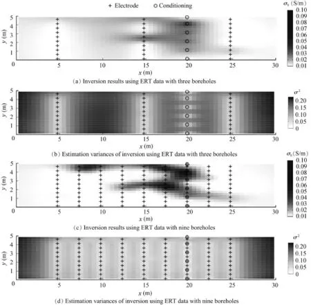
Fig.3.Effect of conditioning at six points in inversion based on SSLE with ERT data at 5%noise level.

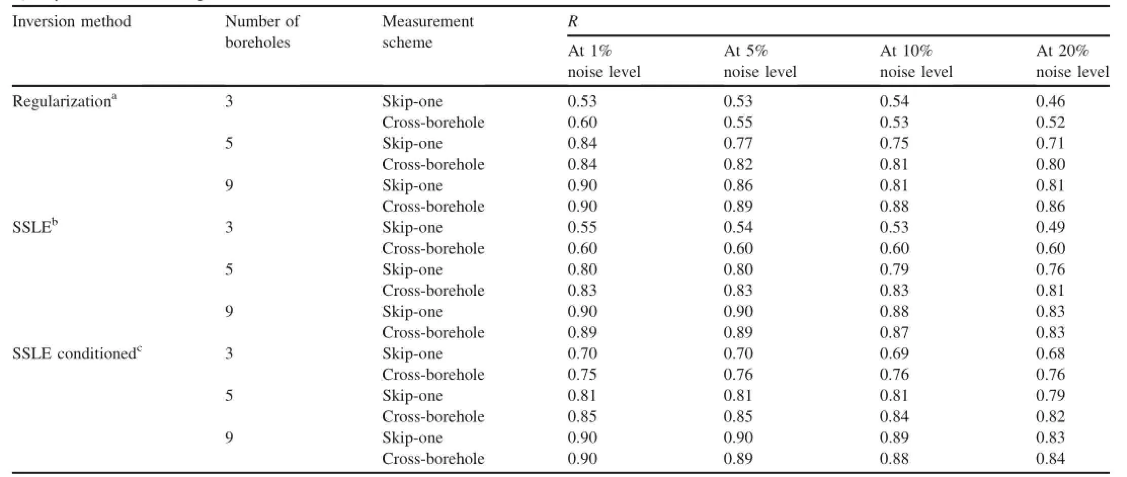
Table1 Quality of inverse modeling.

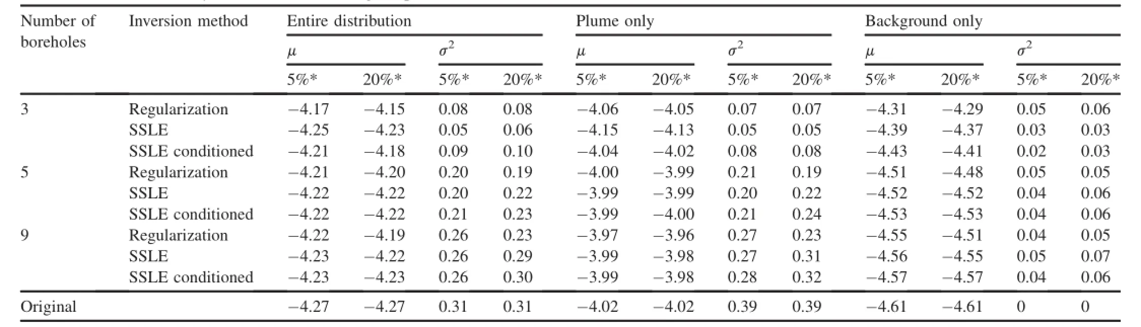
Table2 Bulk electrical conductivity statistics based on original plume and different inversions.

The quality of the estimated electrical conductivity distributions has a signifi cant effect on the inferred plume characteristics:Although the mean electrical conductivity of the estimated plumes is in good agreement with the original plume,even for sparse electrode layouts,the variance of the electrical conductivity is increasingly underestimated with the decreasing number of boreholes(Table 2).The spatial correlation in the vertical direction of the inverted plumes (Figs.4 and 5)shows a less signifi cant decrease with distance when the number of boreholes is reduced.This reflects an increased blurring of the inverted plumes when the number of boreholes is reduced(Fig.2).The spatial correlation in the horizontal direction is only slightly affected by the number of boreholes(Figs.4 and 5).While the first spatial moment, which is a measurement of the location of the center of the plume,is slightly affected by the number of boreholes,the zeroth moment,which is a measurements of the overall solute mass in the plume,is increasingly underestimated when the number of boreholes is reduced(Table 3).The second spatial moment,which is the measurement of the plume extensions in horizontal and vertical directions,is slightly overestimated when the number of boreholes is reduced.

4.2.ERT measurement schemes

A comparison between the skip-one and the cross-borehole measurement schemes in Table 1 shows better inversion results for the given shape of the plume when using the crossborehole measurement scheme.This holds for both inversion approaches.The improvement of the results with the crossborehole measurement scheme is more distinct with use of fewer boreholes.The effect diminishes with an increasing number of boreholes and can be neglected for the SSLE in the nine-borehole layout.Here,using the regularization approach, the cross-borehole measurement scheme still improves the result when dealing with high noise levels.A decrease in R reflects the increasing underestimation of the variance of the electrical conductivity and the zeroth moment of the plume.

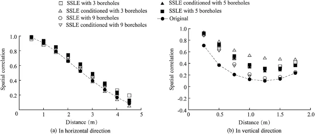
Fig.4.Spatial correlation of original electrical conductivity distribution and inversion results using SSLE and SSLE conditioned methods in cross-borehole measurement scheme at 5%noise level.

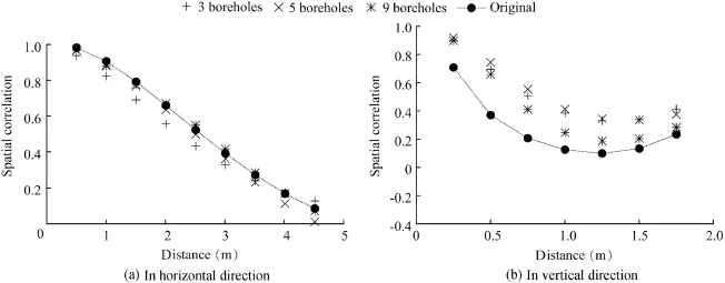
Fig.5.Spatial correlation of original electrical conductivity distribution and inversion results using smoothness-constrained regularization method in cross-borehole measurement scheme at 5%noise level.

4.3.Contrast between plume and background

For a five-borehole layoutat 5%noise leveland use of the cross-borehole measurementscheme we evaluated the effectof different contrasts between plume and background on the quality of the inversion results.We utilized the modified electricalconductivity fields as described atthe end of section 3.1. Furthermore,we ran the same procedures on the modifi ed electrical conductivity fields as pointed out in section 3.2 and analyzed the quality of the results in terms of the correlation coeffi cient,R.

To highlightthe effects of different contrasts,we compared the R values of the inversions based on the modified electrical conductivity fields with those based on the primary electrical conductivity fi eld as presented in Table 1.There the contrast was 10 between the maximum electrical conductivity within the plume and the background electrical conductivity.In Table 4,R values are shown for contrast factors ranging from 1.9 to 46.Comparing the two inversion approaches,SSLE and smoothness-constrained regularization behave similarly with regard to different contrasts.Increasing the contrast to a factor of 19 or even 46 shows no signifi cant change in the quality of the inversion results.However,decreasing the contrast to factors of 1.9,2.8,and 5.5 shows a decrease in R.Although not included in this study,the results suggest that further decrease of the contrast factor leads to even worse estimates.This behavior was to be expected for noisy data since at one point the response of the plume starts to be masked by the noise.On the other hand,the quality of the inversion results is saturated with the increasing contrast between the plume and the background.

4.4.Inversion approaches and their robustness

An integrative comparison of inversion results of the SSLE and the smoothness-constrained regularization approach shows only slight differences in the quality of the results if inputparameters for the inverse procedure are chosen properly(Figs.2,4,and 5,and Tables 1-3).This is in accordance with Kitanidis(1999):“Philosophical differences aside,the stochastic and deterministic approaches share common objectives and may yield similar estimates.”To evaluate the two approaches when the inputparameters are notknown completely but deviate from the correct input parameters,we conducted synthetic ERT experiments using wrong input parameters.We chose the exemplary five-borehole layout with 5%data noise to evaluate the robustness of the two approaches.We found that,for the SSLE approach,the a priori given input of the variance of the electrical conductivity has no significant impact on the quality of the inversion results,at least if the deviation from the true variance is smaller than a bias factor of three.This fi nding was already recognized when the SSLE is used for hydraulic tomography(Yeh and Liu,2000).For the regularization approach,we found thata deviation of the input mean electrical conductivity infl uences the quality of the inversion results in a range of mismatch below a factor of three.

Table3 Spatial moments based on original concentration distribution and different inversion results.

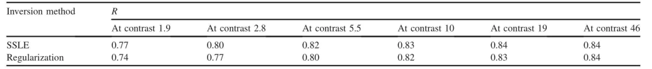
Table4 Quality of inversions with respect to various contrast factors.

However,the results of the SSLE are infl uenced by the a priori given correlation lengths in the horizontal and vertical directions,λhandλv,respectively,as well as the mean of the log-transformed electrical conductivity,μ.The results of the regularization approach are influenced by the a priori given anisotropy ratio,e=λv/λh.Itcan be seen from Table 5 thatboth inversion approaches are quite robustwhen the inputparameters are overestimated,atleastup to a factor of 3.We found thatthe regularization approach was also robust when e was underestimated atleastdown to a factorof0.33.Using the SSLE such robust behavior can only be found for the cross-borehole measurement scheme.For the skip-one measurement scheme,the underestimation of the mean or of all a priori given input parameters together yields results of lower quality(Table 5). These findings indicate that the a priori knowledge of a set of correct statisticalinput parameters as utilized in the SSLE improves the quality of the inversion result only marginally compared to the inversion results based on a smallersetofinput parameters as utilized in the regularization approach(Table 5). On the other hand,the results also suggestthat for reliable estimates of the plume's spatial statistics from ERT inversion results a rough idea ofthe statisticalinputparameters is suffi cient.

4.5.Point conditioning

Using the SSLE,additional information from point measurements of electrical conductivity can be used for point conditioning of the inverse procedure.In Fig.3,the results of inversions including point conditioning are shown together with the estimation variances.Here,in the three-borehole layout the improvement of point conditioning becomes significant.In the nine-borehole layout no improvement can be observed.These results are also expressed in a quantitative way,based on R values in Table 1.No matter which kind of measurementscheme(skip-one orcross-borehole)is used,R is improved by pointconditioning when using a smallnumber of boreholes,but R is only slightly affected by dense electrode layouts.The improvement of the quality of the inverted electrical conductivity distribution by conditioning results in improved estimation of the statistics and spatial moments of the salt plume.This is again more pronounced in layouts with low electrode densities(Tables 2 and 3).

The estimation of the spatial correlation of the inverted electrical conductivity distributions is only slightly improved by point conditioning with the five-and nine-borehole layouts(Fig.4).There is improvement with point conditioning in the three-borehole layout for the correlation in the horizontal direction,but not for the correlation in the vertical direction.In Fig.3(b)the estimation variances are shown for the threeborehole layout.Through point conditioning,the estimation variances are reduced in the area where point measurements are available.The amount of reduction of the estimation variances is highlighted with comparison of the areas around 10 m and around 20 m along the horizontal axis.The same comparison for the nine-borehole layout(Fig.3(d))shows very little difference in estimation variances.This illustrates the improvement through point conditioning with use of only sparse electrode layouts and the diminishing of the improvement with use of dense electrode layouts.

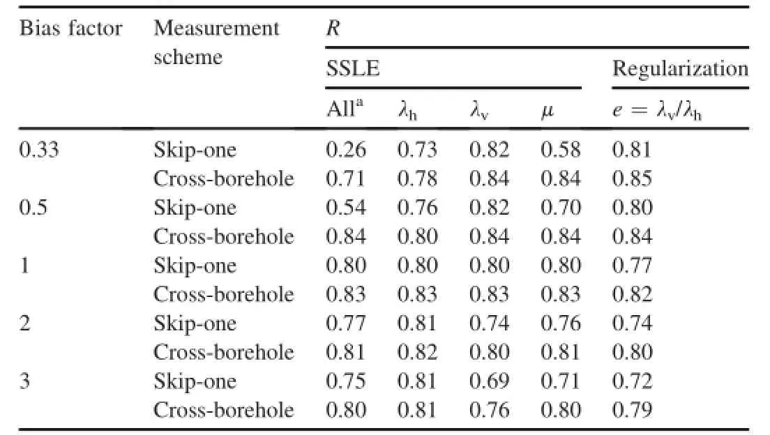
Table5 Influence of incorrect a priori information on inversion results.

5.Conclusions

On the basis of two-dimensional synthetic experiments we simulated ERT cross-borehole surveys and a limited number of point samplings of electrical conductivity for a heterogeneous electrical conductivity distribution representing a salt plume distribution in a heterogeneous aquifer.This study included different ERT layouts,measurement schemes,and inversion approaches.Assuming the relation of electrical conductivity changes against a homogeneous background and concentration to be linear and known,the measurements were utilized to estimate heterogeneous electrical conductivity distributions in order to map the synthetic salt plume.Comparison of the estimated and the true salt plume allowed for an integrated analysis of a geostatistical(SSLE)and a widely used deterministic(smoothness-constrained regularization) inverse modeling approach.This study furthermore provided insights into how ERT inversion results from these two different inversion approaches impact the estimation of salt plume characteristics.Even though various aspects and phenomena may need to be additionally taken into account in real field experiments,the following conclusions from this study can provide understanding of the degree to which the quality of the mapped salt tracer plume depends on the inversion approach for given cross-borehole electrode layouts,noise levels,and conditioning strategies:

Inversions based on the SSLE and smoothness-constrained regularization can provide estimations of plume characteristics of similar quality.Some of the plume characteristics (including the mean concentration,and firstand second spatial moments)can be inferred from ERT surveys more easily. Other characteristics of the salt plumes(i.e.,concentration variance and zeroth spatial moment)cannot be easily inferred from ERT surveys,and success depends on the density and number of electrodes used in the ERT survey.

The choice of the ERT measurement scheme has a significant impact on the quality of the inferred plume characteristics.For the specific geometry of the salt tracer plume considered in this study,the SSLE and the smoothnessconstrained regularization approach yielded better results for the cross-borehole scheme(with a higher signal-to-noise ratio) compared to the commonly used skip-one measurement scheme.In general,the adequacy of a particular measurement scheme depends on the noise level and a compromise between potential resolving power(configurations with large geometric factors)and signal strength(confi gurations with small geometric factors)of the employed measurement confi gurations needs to be found.

The contrast between the salt plume and background electrical conductivity on the one hand,and the noise levelon the other hand,are crucial to the quality of the results of an ERT survey.This suggests thatmapping of high-concentration regions of a plume,as is typically the case in the center of the plume,might still be feasible while low-concentration first arrival and tailing of a plume might be masked by data noise. In this respect,both inversion approaches used in this study showed similar behaviors,i.e.,a decreasing quality of the mapped salt plume with an increasing noise level and with a decreasing level of contrast.

The conditioning by a prioriknown statisticalparameters in both approaches showed only marginal improvement of the inversion results.However,in real-world ERT surveys such statistical parameters are typically unknown and it is thus beneficial that the quality of the mapped salt tracer plumes is only marginally infl uenced by the input parameters of both inversion approaches.The inclusion of in situ point measurements of electrical conductivity(concentration)during the inversion,as shown here for the SSLE,can improve the estimation of plume characteristics signifi cantly,especially if sparse electrode layouts are used.This was also demonstrated by Hermans et al.(2012)in the context of mapping saline intrusion in a coastal aquifer with surface ERT.

Our findings indicate the general potential of integrating differenttypes of data,including geophysicaland hydrological measurements,integraland local(sampling)data,by means of joint inversion procedures for the delineation and characterization of solute plumes.In situations where the geometry of different layers in a groundwater model is known to a reasonable degree,or where modeling with even homogeneous (effective)parameters is justified,the inverse problem can bedirectly formulated in terms of fl ow and transport parameters by coupling the hydraulic model with the geophysicalforward model through an appropriate petrophysical model(Ferrˊe et al.,2009).This way,the inverse solution is inherently forced to respect the physics of the process under investigation,and regularization as in the classical uncoupled deterministic approach is no longer needed.These so-called sequential or coupled hydrogeophysical inversion approaches have seen increasing application over recent years(Kowalsky et al.,2005;Lehikoinen et al.,2009;Beaujean et al.,2014). However,such coupled inversion strategies are also difficultto establish in a feasible manner for cases in which hydraulic heterogeneity is so complex that a model representation in terms of a few zones with constant effective properties is no longer warranted.Therefore,standard uncoupled ERT inversion approaches,like the ones discussed and assessed in this study,will remain important to the imaging and characterization of solute plumes in many real-world applications.

Acknowledgements

We would like to thank J.Beaujean and one anonymous reviewer for their constructive comments,which have improved this manuscript.

Beaujean,J.,Nguyen,F.,Kemna,A.,Antonsson,A.,Engesgaard,P.,2014. Calibration of seawater intrusion models:Inverse parameter estimation using surface electrical resistivity tomography and borehole data.Water Resour.Res.50(8),6828-6849.http://dx.doi.org/10.1002/2013WR014020.

Binley,A.,Henry-Poulter,S.,Shaw,B.,1996.Examination ofsolute transportin an undisturbed soil column using electrical resistance tomography.Water Resour.Res.32(4),763-769.http://dx.doi.org/10.1029/95WR02995.

Binley,A.,Hubbard,S.S.,Huisman,J.A.,Revil,A.,Robinson,D.A.,Singha,K., Slater,L.D.,2015.The emergence of hydrogeophysics for improved understanding ofsubsurface processesovermultiple scales.WaterResour.Res. 51(6),3837-3866.http://dx.doi.org/10.1002/2015WR017016.

Boggs,J.M.,Young,S.C.,Beard,L.M.,Gelhar,L.W.,Rehfeld,K.R., Adams,E.E.,1992.Field study ofdispersion in a heterogeneous aquifer:1. Overview and site description.Water Resour.Res.28(12),3281-3291. http://dx.doi.org/10.1029/92WR01756.

Butler,J.J.,Liu,W.Z.,1993.Pumping tests in nonuniform aquifers:The radially asymmetric case.Water Resour.Res.29(2),259-269.http:// dx.doi.org/10.1029/92WR02128.

Chou,T.K.,Chouteau,M.,Dubˊe,J.S.,2016.Estimation of saturated hydraulic conductivity during infi ltration test with the aid of ERT and level-set method.Vadose Zone J.15(7).http://dx.doi.org/10.2136/vzj2015.05.0082.

Constable,S.C.,Parker,R.L.,Constable,C.G.,1987.Occam's inversion:A practical algorithm for generating smooth models from electromagnetic sounding data.Geophysics 52(3),289-300.http://dx.doi.org/10.1190/ 1.1442303.

Daily,W.,Ramirez,A.,LaBrecque,D.,Barber,W.,1995.Electricalresistivity tomography experiments at the Oregon Graduate Institute.J.Appl.Geophys.33(4),227-237.http://dx.doi.org/10.1016/0926-9851(95)90043-8.

Day-Lewis,F.D.,Singha,K.,Binley,A.M.,2005.Applying petrophysical models to radar travel time and electrical resistivity tomograms: Resolution-dependent limitations.J.Geophys.Res.Solid Earth 110(B8). http://dx.doi.org/10.1029/2004JB003569.

Day-Lewis,F.D.,Chen,Y.,Singha,K.,2007.Moment inference from tomograms.Geophys.Res.Lett.34,L22404.http://dx.doi.org/10.1029/2007 GL031621.

deGroot-Hedlin,C.,Constable,S.,1990.Occam's inversion to generate smooth,two-dimensional models from magnetotelluric data.Geophysics 55(12),1613-1624.http://dx.doi.org/10.1190/1.1442813.

Delleur,J.W.,1999.The Handbook of Groundwater Engineering.CRC Press and Springer Verlag,Boca Raton and Heidelberg.

Ellis,R.G.,Oldenburg,D.W.,1994.Applied geophysicalinversion.Geophys.J. Int.116(1),5-11.http://dx.doi.org/10.1111/j.1365-246X.1994.tb02122.x.

Ferrˊe,T.,Bentley,L.,Binley,A.,Linde,N.,Kemna,A.,Singha,K., Holliger,K.,Huisman,J.A.,Minsley,B.,2009.Critical steps for the continuing advancement of hydrogeophysics.Eos Trans.AGU 90(23), 200.http://dx.doi.org/10.1029/2009EO230004.

Ganz,C.,Bachmann,J.,Noell,U.,Duijnisveld,W.H.M.,Lamparter,A.,2015. Hydraulic modeling and in situ electricalresistivity tomography to analyze ponded infi ltration into a water repellentsand.Vadose Zone J.13(1).http:// dx.doi.org/10.2136/vzj2013.04.0074.

Gottlieb,J.,Dietrich,P.,1995.Identifi cation ofthe permeability distribution in soil by hydraulic tomography.Inverse Probl.11(2),353-360.http:// dx.doi.org/10.1088/0266-5611/11/2/005.

Haarder,E.B.,Jensen,K.H.,Binley,A.,Nielsen,L.,Uglebjerg,T.B., Looms,M.C.,2015.Estimation of recharge from long-term monitoring of saline tracer transportusing electricalresistivity tomography.Vadose Zone J.14(7).http://dx.doi.org/10.2136/vzj2014.08.0110.

Hao,Y.H.,Yeh,T.C.J.,Xiang,J.W.,Illman,W.A.,Ando,K.,Hsu,K.C., Lee,C.H.,2008.Hydraulic tomography for detecting fracture zone connectivity.Groundwater 46(2),183-192.http://dx.doi.org/10.1111/j.1745-6584.2007.00388.x.

Hermans,T.,Vandenbohede,A.,Lebbe,L.,Martin,R.,Kemna,A.,Beaujean,J., Nguyen,F.,2012.Imaging artificial salt water infi ltration using electrical resistivity tomography constrained by geostatistical data.J.Hydrol. 438-439,168-180.http://dx.doi.org/10.1016/j.jhydrol.2012.03.021.

Hermans,T.,Kemna,A.,Nguyen,F.,2016.Covariance-constrained difference inversion of time-lapse electrical resistivity tomography data.Geophysics 81(5),311-322.http://dx.doi.org/10.1190/GEO2015-0491.1.

Illman,W.A.,Berg,S.J.,Zhao,Z.F.,2015.Should hydraulic tomography data be interpreted using geostatisticalinverse modeling?A laboratory sandbox investigation.Water Resour.Res.51(5),3219-3237.http://dx.doi.org/ 10.1002/2014WR016552.

Kemna,A.,2000.Tomographic Inversion of Complex Resistivity:Theory and Application.Ph.D.Dissertation.Ruhr-University of Bochum,Bochum.

Kemna,A.,Vanderborght,J.,Kulessa,B.,Vereecken,H.,2002.Imaging and characterisation of sub-surface solute transport using electrical resistivity tomography(ERT)and equivalent transport models.J.Hydrol.267(3-4), 125-146.http://dx.doi.org/10.1016/S0022-1694(02)00145-2.

Kemna,A.,Binley,A.,Day-Lewis,F.,Englert,A.,Tezkan,B., Vanderborght,J.,Vereecken,H.,Winship,P.,2006.Solute transport processes.In:Vereecken,H.,Binley,A.,Cassiani,G.,Revil,A.,Titov,K., eds.,Applied Hydrogeophysics.NATO Science Series IV:Earth and Environmental Sciences,vol.71.Springer,pp.117-159.http://dx.doi.org/ 10.1007/978-1-4020-4912-5_5.

Kitanidis,P.K.,1999.Generalized covariance functions associated with the Laplace equation and theiruse in interpolation and inverse problems.Water Resour.Res.35(5),1361-1367.http://dx.doi.org/10.1029/1999WR900026.

Koestel,J.,Kemna,A.,Javaux,M.,Binley,A.,Vereecken,H.,2008.Quantitative imaging of solute transport in an unsaturated and undisturbed soil monolith with 3-D ERT and TDR.Water Resour.Res.44(12),W12411. http://dx.doi.org/10.1029/2007WR006755.

Koestel,J.,Vanderborght,J.,Javaux,M.,Kemna,A.,Binley,A., Vereecken,H.,2009a.Noninvasive 3-D transport characterization in a sandy soilusing ERT:1.Investigating the validity of ERT-derived transport parameters.Vadose Zone J.8(3),711-722.http://dx.doi.org/10.2136/ vzj2008.0027.

Koestel,J.,Vanderborght,J.,Javaux,M.,Kemna,A.,Binley,A., Vereecken,H.,2009b.Noninvasive 3-D transport characterization in a sandy soilusing ERT:2.Transportprocess inference.Vadose Zone J.8(3), 723-734.http://dx.doi.org/10.2136/vzj2008.0154.

Korteland,S.A.,Heimovaara,T.,2015.Quantitative inverse modelling of a cylindrical object in the laboratory using ERT:An error analysis.J.Appl. Geophys.114,101-115.http://dx.doi.org/10.1016/j.jappgeo.2014.10.026.

Kowalsky,M.B.,Finsterle,S.,Peterson,J.,Hubbard,S.,Rubin,Y.,Majer,E., Ward,A.,Gee,G.,2005.Estimation of fi eld-scale soil hydraulic and dielectric parameters through joint inversion of GPR and hydrological data.Water Resour.Res.41(11),W11425.http://dx.doi.org/10.1029/ 2005wr004237.

Kraichnan,R.H.,1970.Diffusion by a random velocity field.Phys.Fluids 13(1),22-31.http://dx.doi.org/10.1063/1.1692799.

LaBrecque,D.J.,Miletto,M.,Daily,W.,Ramirez,A.,Owen,E.,1996.The effects of noise on Occam's inversion of resistivity tomography data. Geophysics 61(2),538-548.http://dx.doi.org/10.1190/1.1443980.

LaBrecque,D.J.,Yang,X.J.,2000.Difference inversion of ERT data:A fast inversion method for 3-D in situ monitoring.J.Environ.Eng.Geophys. 6(2),83-89.http://dx.doi.org/10.4133/JEEG6.2.83.

LeBlanc,D.R.,Garabedian,S.P.,Hess,K.M.,Gelhar,L.W.,Quadri,R.D., Stollenwerk,K.G.,Wood,W.W.,1991.Large scale naturalgradient tracer test in sand and gravel,Cape Cod,Massachusetts:1.Experimental design and observed tracer moment.Water Resour.Res.27(5),895-910.http:// dx.doi.org/10.1029/91WR00241.

Lehikoinen,A.,Finsterle,S.,Voutilainen,A.,Kowalsky,M.B.,Kaipio,J.P., 2009.Dynamical inversion of geophysical ERT data:State estimation in the vadose zone.Inverse Problems Sci.Eng.17(6),715-736.http:// dx.doi.org/10.1080/17415970802475951.

Linde,N.,Binley,A.,Tryggvason,A.,Pedersen,L.B.,Revil,A.,2006. Improved hydrogeophysicalcharacterization using jointinversion ofcrosshole electrical resistance and ground-penetrating radar traveltime data. Water Resour.Res.42(12),W12404.http://dx.doi.org/10.1029/2006WR 005131.

Liu,S.Y.,Yeh,T.C.J.,2004.An integrative approach for monitoring water movement in the vadose zone.Vadose Zone J.3(2),681-692.http:// dx.doi.org/10.2113/3.2.681.

Loke, M.H., Wilkinson, P.B., Chambers, J.E., Uhlemann, S.S., Sorensen,J.P.R.,2015.Optimized arrays for 2-d resistivity survey lines with a large numberofelectrodes.J.Appl.Geophys.112,136-146.http:// dx.doi.org/10.1016/j.jappgeo.2014.11.011.

Looms,M.C.,Jensen,K.H.,Binley,A.,Nielsen,L.,2008.Monitoring unsaturated flow and transport using cross-borehole geophysical methods. Vadose Zone J.7(1),227-237.http://dx.doi.org/10.2136/vzj2006.0129.

Mackay,D.M.,Freyberg,D.L.,Roberts,P.V.,Cherry,J.A.,1986.A natural gradientexperimenton solute transportin a sand aquifer:1.Approach and overview of plume movement.Water Resour.Res.22(13),2017-2029. http://dx.doi.org/10.1029/WR022i013p02017.

Moysey,S.,Singha,K.,Knight,R.,2005.A framework for inferring fieldscale rock physics relationships through numerical simulation.Geophys. Res.Lett.32(8).http://dx.doi.org/10.1029/2004GL022152.

Mu¨ller,K.,Vanderborght,J.,Englert,A.,Kemna,A.,Huisman,J.A.,Rings,J., Vereecken,H.,2010.Imaging and characterization of solute transport during two tracer tests in a shallow aquifer using electrical resistivity tomography and multilevelgroundwater samplers.Water Resour.Res.46(3), W03502.http://dx.doi.org/10.1029/2008WR007595.

Neuendorf,O.,1996.Numerische 3-D Simulation des Stofftransportes in einem Heterogenen Aquifer.Ph.D.Dissertation.RWTH Aachen,Aachen.

Nguyen,F.,Kemna,A.,Antonsson,A.,Engesgaard,P.,Kuras,O.,Ogilvy,R., Gisbert,J.,Jorreto,S.,Pulido-Bosch,A.,2009.Characterization of seawater intrusion using 2D electrical imaging.Near Surf.Geophys. 7(5-6),377-390.http://dx.doi.org/10.3997/1873-0604.2009025.

Persson,M.,Dahlin,T.,Gu¨nther,T.,2015.Observing solute transport in the capillary fringe using image analysis and electrical resistivity tomography in laboratory experiments.Vadose Zone J.14(5).http://dx.doi.org/10.2136/ vzj2014.07.0085.

Pidlisecky,A.,Singha,K.,Day-Lewis,F.D.,2011.Distribution-based parametrization for improved tomographic imaging of solute plumes. Geophys.J.Int.187(1),214-224.http://dx.doi.org/10.1111/j.1365-246X.2011.05131.x.

Revil,A.,Karaoulis,M.,Johnson,T.,Kemna,A.,2012.Review:Some lowfrequency electrical methods for subsurface characterization and monitoring in hydrogeology.Hydrogeology J.20(4),617-658.http:// dx.doi.org/10.1007/s10040-011-0819-x.

Rubin,Y.,Hubbard,S.S.,2005.Hydrogeophysics,first ed.Springer, Dordrecht.

Seidemann,R.,1996.Parallelisierung eines Finite Elemente Programms zur Modellierung des Transports von Stoffen durch Heterogene Por¨ose Medien.Ph.D.Dissertation.Rheinische Friedrich-Wilhelms-Universit¨at Bonn, Bonn.

Singha,K.,Gorelick,S.M.,2005.Saline tracer visualized with threedimensional electrical resistivity tomography:Field-scale spatial moment analysis.Water Resour.Res.41(5),W05023.http://dx.doi.org/10.1029/ 2004WR003460.

Singha,K.,Day-Lewis,F.D.,Johnson,T.,Slater,L.D.,2015.Advances in interpretation of subsurface processes with time-lapse electrical imaging. Hydrol.Processs 29(6),1549-1576.http://dx.doi.org/10.1002/hyp.10280.

Slater,L.,Binley,A.,Versteeg,R.,Cassiani,G.,Birken,R.,Sandberg,S., 2002.A 3D ERT study of solute transportin a large experimental tank.J. Appl. Geophys. 49(4), 211-229. http://dx.doi.org/10.1016/S0926-9851(02)00124-6.

Vanderborght,J.,2001.Concentration variance and spatial covariance in second-order stationary heterogeneous conductivity fields.Water Resour. Res.37(7),1893-1912.http://dx.doi.org/10.1029/2001WR900025.

Vanderborght,J.,Kemna,A.,Hardelauf,H.,Vereecken,H.,2005.Potentialof electrical resistivity tomography to infer aquifer transport characteristics from tracer studies:A synthetic case study.Water Resour.Res.41(6), W06013.http://dx.doi.org/10.1029/2004WR003774.

Vereecken,H.,Lindenmayr,G.,Neuendorf,O.,D¨oring,U.,Seidemann,R., 1994.Trace a Mathematical Model for Reactive Transport in 3D Variably Saturated Porous Media.Tech.rep.,KFA-ICG-4-501494,Ju¨lich.

Vereecken,H.,Neuendorf,O.,Lindenmayr,G.,Basermann,A.,1996.A Schwarz domain decomposition method for solution of transient unsaturated water fl ow on parallel computers.Ecol.Model.93(1-3),275-289. http://dx.doi.org/10.1016/0304-3800(95)00224-3.

Vereecken,H.,D¨oring,U.,Hardelauf,H.,Jaekel,U.,Hashagen,U., Neuendorf,O.,Schwarze,H.,Seidemann,R.,2000.Analysis of solute transport in heterogeneous aquifer:The Krauthausen field experiment.J. Contam.Hydrol.45(3-4),329-358.http://dx.doi.org/10.1016/S0169-7722(00)00107-8.

Vereecken,H.,Binley,A.,Cassiani,G.,Revil,A.,Titov,K.,2006.Applied Hydrogeophysics.Springer,pp.1-9.

Wu,C.M.,Yeh,T.C.J.,Zhu,J.,Lee,T.H.,Hsu,N.S.,Chen,C.H.,Sancho,A.F., 2005.Traditional analysis of aquifer tests:Comparing apples to oranges? Water Resour.Res.41(9),W09402.http://dx.doi.org/10.1029/2004WR 003717.

Yeh,T.C.J.,Liu,S.,2000.Hydraulic tomography:Development of a new aquifer test method.Water Resour.Res.36(8),2095-2105.http:// dx.doi.org/10.1029/2000WR900114.

Yeh,T.C.J.,Liu,S.,Glass,R.,Baker,K.,Brainard,J.,Alumbaugh,D., LaBrecque,D.,2002.A geostatistically based inverse model for electrical resistivity surveys and its applications to vadose zone hydrology.Water Resour.Res.38(12),1278.http://dx.doi.org/10.1029/2001WR001204.

Yeh,T.C.J.,Zhu,J.,Englert,A.,Guzman,A.,Flaherty,S.,2006.A successive linear estimator for electrical resistivity tomography.In:Vereecken,H., Binley,A.,Cassiani,G.,Revil,A.,Titov,K.,eds.,Applied Hydrogeophysics.Springer,pp.45-74.

Zhu,J.,Yeh,T.C.J.,2005.Characterization of aquifer heterogeneity using transienthydraulic tomography.Water Resour.Res.41(7),W07028.http:// dx.doi.org/10.1029/2004WR003790.

Zimmerman,D.A.,de Marsily,G.,Gotway,C.A.,Marietta,M.G., Axness,C.L.,Beauheim,R.L.,Bras,R.L.,Carrera,J.,Dagan,G., Davies,P.B.,et al.,1998.A comparison of seven geostatistically based inverse approaches to estimate transmissivities for modeling advective transport by groundwater flow.Water Resour.Res.34(6),1373-1413. http://dx.doi.org/10.1029/98WR00003.

Andreas Englerta,*,Andreas Kemnab,Jun-feng Zhuc,Jan Vanderborghtd,Harry Vereeckend, Tian-Chyi J.Yehe,f

aInstitute of Geology,Mineralogy and Geophysics,Ruhr University Bochum,Bochum D-44801,Germany
bDepartment of Geophysics,Steinmann Institute,University of Bonn,Bonn D-53115,Germany
cKentucky Geological Survey,University of Kentucky,Lexington KY-40506,USA
dAgrosphere,Institute for Bio-and Geosciences(IBG-3),Forschungszentrum Ju¨lich GmbH,Ju¨lich D-52425,Germany
eDepartment of Resources Engineering,National Cheng Kung University,Tainan TW-701,China
fDepartment of Hydrology and Water Resources,The University of Arizona,Tucson AZ-85721,USA

Received 30 December 2015;accepted 11 September 2016

Available online 18 January 2017

*Corresponding author.

E-mail address:andreas.englert@rub.de(Andreas Englert).

Peer review under responsibility of Hohai University.

?2016 Hohai University.Production and hosting by Elsevier B.V.This is an open access article under the CC BY-NC-ND license(http:// creativecommons.org/licenses/by-nc-nd/4.0/).