Fast High Order and Energy Dissipative Schemes with Variable Time Steps for Time-Fractional Molecular Beam Epitaxial Growth Model

Dianming Hou ,Zhonghua Qiao and Tao Tang

1 School of Mathematics and Statistics,Jiangsu Normal University,Xuzhou,Jiangsu 221116, China

2 Department of Applied Mathematics, The Hong Kong Polytechnic University, Hung Hom, Kowloon, Hong Kong, China

3 Guangdong Provincial Key Laboratory of Interdisciplinary Research and Application for Data Science, BNU-HKBU United International College,Zhuhai, Guangdong 519087, China

Abstract.In this paper,we propose and analyze high order energy dissipative time-stepping schemes for time-fractional molecular beam epitaxial (MBE)growth model on the nonuniform mesh.More precisely,(2-α)-order,secondorder and (3-α)-order time-stepping schemes are developed for the timefractional MBE model based on the well known L1,L2-1σ,and L2 formulations in discretization of the time-fractional derivative,which are all proved to be unconditional energy dissipation in the sense of a modified discrete nonlocalenergy on the nonuniform mesh.In order to reduce the computational storage,we apply the sum of exponential technique to approximate the history part of the time-fractional derivative.Moreover,the scalar auxiliary variable (SAV)approach is introduced to deal with the nonlinear potential function and the history part of the fractional derivative.Furthermore,only first order method is used to discretize the introduced SAV equation,which will not affect high order accuracy of the unknown thin film height function by using some proper auxiliary variable functions V(ξ).To our knowledge,it is the first time to unconditionally establish the discrete nonlocal-energy dissipation law for the modified L1-,L2-1σ-,and L2-based high-order schemes on the nonuniform mesh,which is essentially important for such time-fractional MBE models with low regular solutions at initial time.Finally,a series of numerical experiments are carried out to verify the accuracy and efficiency of the proposed schemes.

Key words: Time-fractional molecular beam epitaxial growth,variable time-stepping scheme,SAV approach,energy stability.

1 Introduction

The technique of molecular beam epitaxy (MBE) is among the most refined methods for the growth of thin solid films and is of great importance for applied studies.It allows to grow high-quality crystalline films,and form structures with high precision in the vertical direction,such as monolayer-thin interfaces or atomically flat surfaces.The macroscopic evolution of the growing film is directly related to movement of adatoms on surfaces and their various bonding configurations,thus it is attractive to use atomic-scale simulations for a theoretical description of epitaxial growth.However,in order to reach the length and time scales of interest for various applications,the continuous models have to be used.Several different types of MBE models including atomistic models [9,24],continuum models [26,48],and hybrid models[6,14],have been derived and investigated to better understand the thin film growth mechanisms behind its technological applications.Among these models,the continuum model has been attracting particular interest in the community by modeling the epitaxial growth via partial differential equations with structure of gradient flow:

whereφis a scaled height function of the thin film,Mrepresents a positive mobility parameter,andis functional derivative in term of a total free energyE(φ) inL2sobolev space.It is worth to mention that the above MBE model (1.1) satisfies the following energy dissipation law

where (·,·) denotes theL2-inner product,and‖·‖is the associated norm.For the MBE model (1.1),there exists a huge amount of numerical work preserving the dissipation energy law (1.2)or a mild modified version in discrete lever;see,e.g.,[8,12,23,37,38,44,49,51].

In recent years,time-fractional gradient flow models have attracted increasingly attention[1–3,10,11,19,28,34,45,54].The so-called fractional derivative involved in the gradient flows can be regarded as an average of the traditional derivative with some weighted kernel functions in the history process.It leads to the current phase transition in time depending on the ones at all previous times,which makes the timefractional model gain more advantages over the traditional one in modeling some viscoelastic materials or polymers with memory effects.In this work,we numerically investigate the typical time-fractional MBE model [7,21,52] as follows:

and the corresponding total free energy is given by

Hereεis a positive constant controlling the surface diffusion strength,andF(?φ)=(|?φ|2-1)2is double-well potential for the model(1.3)with slope selection.Then,the governed equation (1.3) for the height functionφreads

is functional derivative ofF(?φ).

There exists an amount of numerical works for the time-fractional gradient flow models.Among the existing studies on this type of models,Wang and his collaborators developed efficient numerical schemes for time fractional phase-field models in[7,34,53].They numerically investigated the anomalously sub-diffusive transport behavior in heterogeneous porous materials or memory effects of certain materials.The numerical results showed that the coarsening dynamic scaling law for the energy of the time fractional Cahn-Hilliard and MBE model decayed aswhich has been theoretically proved in a very recent work [46].Tang et al.proved that the time-fractional phase field model admits an integral type energy dissipation law for the first time in[47].Moreover,in their work,an efficient L1 time stepping schemes has been developed for typical time fractional phase field models preserving this type of energy law in discrete sense on the uniform temporal mesh.In [11],Du et al.have proved the well-posedness,maximum principle,and the solution regularity for the time fractional Allen-Cahn equation.They constructed several time stepping schemes based on weighted convex splitting scheme and linear stabilized scheme,and showed that the error of the proposed numerical schemes are of orderαfor the uniform mesh without any solution regularity assumptions.Recently,Quan et al.theoretically proved that the time-fractional derivative of the original energy is always nonpositive for time-fractional gradient flows in [40].Moreover,a weighted energy dissipation law was also derived for this type of models under a restriction on the weight function.Accordingly,a first order numerical scheme has been constructed for time-fractional gradient flow [41] preserving the weighted energy dissipation law in discrete level.Recently,an adaptive second-order timestepping scheme based on the Crank-Nicolson(CN)formula and the scalar auxiliary variable (SAV) approach was developed and analyzed for the time-fractional MBE growth model in [21].The proposed scheme are proved to be unconditionally stable in the sense that the modified discrete energy can be bounded by the initial free energy.In [16–18],a nonlocal energy dissipation law was derived for the timefractional phase field models with any given temporal mesh.Based on this nonlocal energy dissipation law,the high order and efficient linear time stepping schemes were developed for the time-fractional Allen-Cahn and MBE equations using SAV approach.In particular,the proposed schemes base on the Crank-Nicolson formula in [16] were proved unconditionally stable for quite general meshes.However,the stabilities of the high order numerical schemes based on the L1,L2-1σ,and L2 formulations in [17,18] were only proved for the uniform temporal meshes.It seems rather difficult to theoretically establish the stabilities of the proposed L1 and L2 based schemes on the nonuniform mesh even for a modified free energy.Very recently,another type of nonlocal-in-time modified energy dissipation law was obtained in [39] for the time-fractional Allen-Cahn equation.The proposed nonlocal modified energy is an upper bound of the traditional original free energy,and coincides the original energy at initial time andt →∞.Furthermore,L1 and L2 stabilized schemes were developed for the time-fractional Allen-Cahn equation,and proved to be unconditionally stable in the sense of a similar modified energy decreasing on the uniform temporal mesh.Very recently,the global–in–time H1-stabilities of L2-1σand L2 schemes have been successfully obtained in [42,43] for the linear subdiffusion equation on the nonuniform temporal mesh with the time step ratioγnno less than 0.4753 and 0.4573≤γn ≤3.5615,respectively.The positive semidefiniteness of the bilinear form associated with the L2-1σand L2 formulas were derived under such restrictions on the time step ratios.In recent work [27],Li and Liao used the technique of the discrete orthogonal convolution (DOC) kernels to obtain that the two–step backward differentiation formula (BDF2) method is stable on arbitrary time grids and the variable time–step BDF3 method is stable if the adjacent step ratios are less than 2.553.It is worth to mention that there seems to be no high order energy dissipative schemes for time-fractional MBE model (1.6) based on L1,L2-1σ,and L2 formulations on the nonuniform mesh.

The time fractional derivative(1.4)involved in these types of phase-field models will lead to the low regularities of the solutions abouttαat the initial time,which has been numerically proved in [11,16,17,21].In this case,using uniform temporal mesh may result in a loss of convergence order for the proposed high order numerical method,thus it is particularly important to construct higher-order unconditionally energy-dissipative schemes for this type of models on the non-uniform grid meshes,which can help recover the optimal convergence rate of the proposed high-order schemes by refining the temporal mesh according to the initial regularity of the solution.One of non-uniform meshes for this type of the fractional model,probably the most used,is the so-called graded mesh defined by

whereTis the terminal time andNdenotes the number of subintervals in [0,T].Moreover,coarsening dynamic process of the time fractional MBE model usually requires long time simulation,in which the free energy usually undergoes large changes in some time intervals,but varies little during some other time intervals.Thus,it is highly desirable to develop high order and unconditionally energy-stable linear schemes with variable time steps for the time-fractional MBE model (1.6).Therefore,the graded mesh and the existing time-adaptive strategies can be easily applied to improve the accuracy and efficiency of the proposed high order numerical schemes.The main purpose of this paper is to develop linear,high-order,and unconditionally energy-stable schemes with variable time steps that preserve the nonlocal energy dissipation law obtained in [17] in the discrete level.The main idea is to use the scalar auxiliary variable (SAV) approach to deal with the history part term of the fractional derivative and the nonlinear potential functionf(?φ),and meanwhile adopt a first-order method to discretize the SAV equation.This will play an important role in unconditionally deriving the discrete nonlocal-energy dissipation law of the constructed high-order schemes based on the modified L1,L2-1σ,and L2 formulations on the nonuniform mesh.Moreover,a fast evaluation technique based on the sum-of-exponentials approach[22]is used to accelerate the calculation of the history part of the fractional derivative and reduce the corresponding storage.

The paper is organized as follows: In the next section,we give a brief review on the nonlocal energy dissipation law obtained in [17] for the time-fractional MBE model (1.6) and construct the equivalent SAV reformulation of the corresponding continuous problem.The fast finite difference operators for the discretization of the fractional derivative are developed base on the SOE technique.In Section 3,we propose the modified fast L1-SOE,L2-1σ-SOE and L2-SOE schemes for the equivalent SAV reformulation system of the model (1.6),and carry out the corresponding discrete nonlocal energy dissipation law for the proposed high-order linear schemes.Several numerical experiments are carried out in Section 4,not only to validate the stability and accuracy of the proposed methods,but also to numerically investigate the coarsening dynamics of the time-fractional MBE growth models.Finally,the paper ends with some concluding remarks.

2 Nonlocal energy dissipation law and SAV reformulation

Without loss of generality,in what follows,we consider the time-fractional MBE model (1.6) withM=1 on a bounded domain Ω∈Rn(n=1,2,3),equipped with periodic boundary conditions.

2.1 Nonlocal energy dissipation law

For any given temporal mesh 0=t0＜t1＜t2＜···＜tN=T,the time-fractional MBE model (1.6) satisfies the following nonlocal energy equation [17,18]:

We integrate(2.1)fromtntotn+1to obtain the following nonlocal energy dissipation law:

For the negativity of the last term,one can refer [16,21,47].

for alln=0,1,...N-1.As of now,it is still an open issue whether the original energyE(φ) is dissipative in time or not for this type of gradient flow,which may require more effort to make it clear in the future.Our goal of introducing the nonlocal energy is to construct schemes,which are unconditionally stable in the sense that the modified discrete nonlocal energy remains bounded during the time-stepping with a lower bound assumption on(φ).

2.2 SAV reformulation

Inspired by the idea of a variant of SAV approach introduced in [15],we introduce a scalar auxiliary variableR(t),defined by

where

andC0is a positive constant.Throughout this paper,we will assume that(φ)is bounded from below,i.e.,there always exists a positive constantC0such thatE(φ)+C0＞0.Then the time-fractional MBE model (1.6) can be rewritten into following equivalent form,for anyt∈[tn,tn+1],

andV(ξ) is a real function with respect toξsuch thatV(1)=1.

2.3 Fast finite difference operators for time-fractional derivative

In this subsection,we recall several finite difference operators for the discretization of the Caputo fractional derivative with SOE technique [22,55],including the classical(2-α)-order L1 formulation and two kinds of (3-α)-order operators including the L2-1σand L2 formulations.These fast schemes make use of the liner interpolation or the quadratic interpolation of the unknown function for the local part of the fractional derivative,and adopt the SOE approach to discretize the history partPrecisely,we define the linear interpolation operator Π1,jφ(t),j=0,...,N-1,by

and the quadratic interpolation operator Π2,jφ(t)fort∈[tj-1,tj+1]andj=1,2,...,N-1,by

Then we use the linear interpolation to obtain the discretization of the local fractional partφwithtn+σ:=tn+στn+1,σ∈(0,1]:

It has been proved;see,e.g.,[13,35],that=O(τ3-α),provided the solution is smooth enough in time.

For the history partφof the fractional derivative withσ ∈(0,1],taking the integration by part gives

with 0＜δ ?1.This is the so-called sum-of-exponentials technique to approximate the singular kernel function 1/tρ.Thus the history term can be evaluated via the SOE technique,that is,

By utilizing a recursive formula and the interpolation operations defined in (2.6)and (2.7),Ui,h(tn+σ) can be further approximated by,forn=1,...,N-1 withk=1,andn=2,...,N-1 withk=2,

Thus,the fast finite difference operator to discretize the history partof the fractional derivative is obtained as follows: forn=1,...,N-1 whenk=1,andn=2,...,N-1 in the case ofk=2,

Starting with the equivalent SAV reformulation(2.5)and the fast finite difference operators for the discretization of the fractional derivative,we are ready to construct various time stepping schemes to numerically calculate the solutionφ.

3 Fast higher order SOE schemes on the nonuniform temporal mesh

In this section,we construct and analyze several high order numerical schemes for the time-fractional MBE model (1.6),including fast modified L1,L2-1σand L2 schemes using the SAV approach.

3.1 Fast 2-α order L1-SOE scheme

Using the proposed fast finite difference operators defined in (2.8) and (2.12) withσ=1 andk=1,we obtain the following 2-αorder scheme for the equivalent system(2.5) on the nonuniform temporal mesh,forn=1,2,···,N-1,

whereφ*,n+1:=φn+γn+1(φn-φn-1) is an explicit second-order approximation toφ(tn+1).We call it the fast L1-SOE scheme,hereafter.

It seems that the above proposed fast modified L1-SOE scheme is of first order accuracy forφ,since the first order BDF approach is used to discretize the auxiliary variable equation(3.1b).However,this treatment for(3.1b)will not affect the 2-αorder accuracy of the unknown functionφ,and plays a crucial role in the derivation of energy dissipative stability of the fast modified L1-SOE scheme (3.1) on the nonuniform temporal mesh,if we carefully choose the auxiliary variable functionV(ξ) such that

Then,we use the Taylor expansion ofξV(ξ) atξ=1 to derive that

withξ=1+O(τ),seeing also[15].Therefore,althoughξn+1is solved from(3.1b)and(3.1c) with only first-order accuracy,ξn+1V(ξ) in (3.1a) is of second-order in time and will not affect the (2-α)-th order of the phase functionφ.In fact,there exist several types of the auxiliary functionV(ξ)satisfying(3.2),such as 2-ξ,exp(1-ξ),1+sin(1-ξ),and so on.

The stability property of the scheme is stated in the following theorem.

Theorem 3.1.For the general temporal mesh,the fast modified L1-SOE scheme(3.1)is unconditionally energy stable in the sense of

where

Proof.Taking theL2–inner products of(3.1a)withφn+1-φn,and Multiplying(3.1b)with 2Rn+1τn+1,gives

Then we sum the above two equations up,use the following identity

and drop some non-essential positive terms to obtain

Then we end the proof.

Next,we show how to efficiently solve the fast modified L1-SOE scheme (3.1).It follows from (3.1a) that

Then,it is easy to see that+can be viewed as a numerical solution ofφ(tn+1) solved by the traditional 2-αorder linear stabilized method for the timefractional MBE model (1.6).Substituting (3.6) and (3.1c) into (3.1b),we obtain a nonlinear algebraic equation with respect toξn+1:

Denoting the left side of the above equation byW(ξn+1),and together withV(1)=1 andV′(1)=-1,we have the following identities

Thus,ξn+1can be efficiently evaluated by solving the nonlinear algebraic equation(3.8) using the Newton’s iteration with the initial conditionξ0=1,and it will converge quickly with a large enoughC0.

In detail,the fast modified L1-SOE scheme (3.1) results in the following algorithm at each time step:

(i) Evaluation ofandfrom(3.7a)and(3.7b)respectively,which can be realized in parallel.

(ii) Calculation ofξn+1using Newton’s iteration method for (3.8),and thenφn+1can be obtained by (3.6).

The total computational complexity at each time step is essentially that of solving two bi-Laplacian equations with constant coefficients,since the computational cost for solving the nonlinear algebraic problem (3.8) by Newton’s iteration can be negligible compared to the cost of solvingand

3.2 Fast modified L2-1σ-SOE and L2-SOE schemes

In this subsection,we develop and investigate several high-order,unconditionally energy-dissipative schemes for the time-fractional MBE model (1.6) with the fast difference operators defined in Subsection (2.3).

3.2.1 Fast second-order modified L2-1σ-SOE scheme

Using the fast difference operatorsandwithσ=1-α/2 to discretize the fractional derivative,we derive the following fast second-order modified L2-1σ-SOE scheme for the equivalent system (2.5) withn=1,2,···,N-1,

are of second-order implicit and explicit approximations toφ(tn+1),respectively.

The stability property of the fast modified L2-1σ-SOE scheme(3.10)is presented in the following theorem.

Theorem 3.2.For the general temporal mesh,the fast modified L2-1σ scheme(3.10)is unconditionally energy stable in the sense of

whereis defined in(3.4).

Proof.We take theL2–inner products of (3.10a) withφn+1-φn,and meanwhile multiply (3.10b) with 2Rn+1τn+1,to obtain

It follows from the identity (3.5) andσ=1-α/2 that

Furthermore,summing (3.12a) and (3.12b) up,and using the identity (3.5) and(3.13),gives

Then,we remove some non-essential positive terms from the above equality and note the definition ofin (3.4),to obtain the desired unconditional stability (3.17).Thus,we end the proof.

3.2.2 Fast second-order modified L2-SOE scheme

Using the fast difference operatorsandto discretize the fractional derivative,we derive the following fast second-order modified L2-SOE scheme for the equivalent system (2.5) withn=1,2···,N-1,

whereφ*,n+1is defined in (3.1).

Before proving the stability of the scheme,some preparations are needed.We first introduce the following two-variable function:

whereg1(s) andg2(z) are given respectively by

Then,we can derive thatG(s,z) is increasing in (0,s*(α)) and decreasing in(s*(α),+∞) with respect tos,wheres*(α) is the positive extreme point ofg1depending onα.It is easy to check thatG(s,z) is decreasing with respect toz.Moreover,for eachα ∈(0,1),there exists a positive real numberγ*(α) such thatG(γ,γ) is increasing in (0,γ*(α)) and decreasing in (γ*(α),+∞).Letγ**(α) be the positive root of the equationG(γ,γ)=0,sinceG(0,0)=2(2-α)＞0 andG(γ,γ)→-∞asγ →+∞.Noting

where we have used thatg(α):=2(2-α)+8α(1-22-α)/5 is decreasing with respect toα∈(0,1) andg(1)=2/5.Then we have 0＜γ*(α)＜4＜γ**(α).Moreover,we haveG(0,z)≥G(4,z) forz ∈(0,∞),then one can derive

for all 0＜s,z≤γ**(α).The following lemma is essential importance in the derivation of the energy dissipation of the fast second-order modified L2-SOE scheme (3.14).

Lemma 3.1.For the temporal mesh with0＜γn+1≤γ**(α),n=1,...,M-1,it holds

Proof.We use the definitions ofin (2.9),and the inequality-2ab≥-a2-b2to deduce that

Then the desired result (3.16) follows from combining the above estimate with the inequality (3.15).

The stability property of the fast modified L2-SOE scheme (3.14) is stated in the following theorem.

Theorem 3.3.For the general temporal mesh,the fast second-order modified L2 scheme(3.14)is unconditionally energy stable in the sense of

withdefined by

whereis given in(3.4).

Proof.Since the proving process is similar to the one of Theorem 3.1 by using Lemma 3.1,we omit the proof detail and leave it for interested readers.

Remark 3.1.With the same treatment for the auxiliary variable equation (2.5b),one can also develop a 3-αorder unconditionally energy-stable modified L2 scheme by setting the auxiliary variable functionV(ξ) such that

Using the Taylor expansion ofξV(ξ) atξ=1 gives

withξ=1+O(τ).Then,we have

which will not affect the (3-α)-order accuracy ofφwith first order treatment for(3.14b).

Remark 3.2.Noting that theH1-stability of the L2-1σand L2 schemes for the linear subdiffusion equation on general nonuniform meshes have been successfully established in recent works [42,43],via proving positive semidefiniteness of the discrete bilinear form associated with the L2-1σand L2 formulas with a mild restriction on the step-ratiosγn.A lower bound of the time-step ratios (γn ≥0.4753 for L2-1σformula andγ ≥4/7 for L2 formula) is needed in the derivation of the positive semidefiniteness of the corresponding discrete fractional-derivative operator,which seems to be only a sufficient condition of theH1-stability for the proposed numerical schemes to ensure the positive semidefiniteness of the discrete bilinear form.For the classic multi-step method (BDF-k,1≤k ≤5),one can use a weak result to derive the stability and corresponding error analysis of the numerical scheme,that is the gradient stability of the BDF–k formulas (1≤k≤5) [20,25,30–32,36].Furthermore,the gradient stability and the positive semidefiniteness of the BDF-2 formula with variable time steps have been successfully obtained with the step-ratiosγn ＜4.8645 in Lemma 2.1 of [29],and the variable-step BDF–3 formula scheme is stable when the step ratios are less than 2.553 in [27].The condition of lower bound restriction onγnin [42,43] may be able to be improved or removed by using some special technique such as the technique of the discrete orthogonal convolution (DOC) kernels used in [27],since the L2-1σand L2 formulas will converge to Crank-Nicolson(positive defined) and BDF-2 formulas with variable time steps,respectively,whenα→1.In our derivation of the stability results of the modified L2-1σand L2 schemes in Theorems 3.2 and 3.3,we only use the positive semidefiniteness of the local partand the gradient stability (3.16) of the local partrespectively,where the history partsξn+1V(ξn+1)k,k=1,2 are modified approximate versions of the standard ones.This leads to the stability of the proposed schemes only requiring 0＜γn+1≤γ**(α),n=1,...,M-1,without a lower bound on the time-step ratios.

Moreover,it is worth pointing out that all of the above proposed high-order numerical schemes can be efficiently implemented by following the similar lines of the Algorithm (i)-(ii) in the previous subsection.

4 Numerical results

In this section,several numerical experiments are provided to demonstrate the accuracy and stability of the proposed high-order fast schemes for the time-fractional MBE model (1.6).We always chooseV(ξ)=1+sin(1-ξ) for no more than secondorder schemes,andV(ξ)=3-3ξ+ξ2for 3-αorder schemes in the numerical tests,such that the conditions (3.2) and (3.18) are satisfied,respectively.The stabilizing parameter is set to bes=1 throughout the following numerical experiments.Furthermore,in order to guarantee the positivity of+C0and the convergence of the Newton’s iteration for the nonlinear algebraic equation at each time step,we always setC0=1e16 to be large enough unless specified othwise.Since the time-fractional MBE model (1.6) considered in this work is subject to the periodic boundary condition,the Fourier spectral method is applied for spatial discretization.

4.1 Convergence order test

Example 4.1.Consider the following time fractional MBE model:

wheres(x,t) is a fabricated source term such that the exact solution is

In this test,we use Fourier spectral method with large enough 128×128 modes for the spatial discretiztion to ensure that the spatial discretization error can be negligible compared to the temporal one.Due to the exact solution of this testing example is smooth in time,we only investigate convergence orders of the modified L1-SOE,L2-1σ-SOE and L2-SOE scheme on the uniform temporal mesh.The corresponding errors are measured by the maximum norm,that is,

In Fig.1,the errors up toT=0.1 as functions of the time step sizes are plotted in log-log scale for the proposed schemes.It is shown that all the tested numerical schemes achieve the desired convergence order on the uniform mesh.That is,the modified L1-SOE scheme (3.1) achieves a convergence rate of 2-αorder;both the modified L2-1σ-SOE (3.10) and the modified L2-SOE schemes (3.14) are of secondorder accuracy;while the modified L2-SOE scheme discussed in Remark 3.1 obtains the desired 3-αorder accuracy.

Example 4.2.Consider the equation (1.6) in the domain (0,2π)2×(0,T] with the initial dataφ(x,0)=0.1(sin3xsin2y+sin5xsin5y) andε2=0.01.

Due to the time-fractional derivative involved in the MBE model,the solution of (1.6) usually behaves a low regularity abouttαat the initial time,which has been numerically reported in [11,16,17,21].In this example,we again numerically investigate the initial behaviors of the solution by our proposed fast high order schemes,and demonstrate how to recover the optimal convergence order of the proposed schemes via refining the temporal grids.Again,the Fourier method is used for the spatial discretization with 128×128 modes,and the so-called graded mesh defined in (1.7) withT=0.1 andN=10×2k,k=1,2,···10 is used for all the tested numerical schemes withC0=100.Since the exact solution is unknown,we evaluate the errors of numerical solutions as follows:

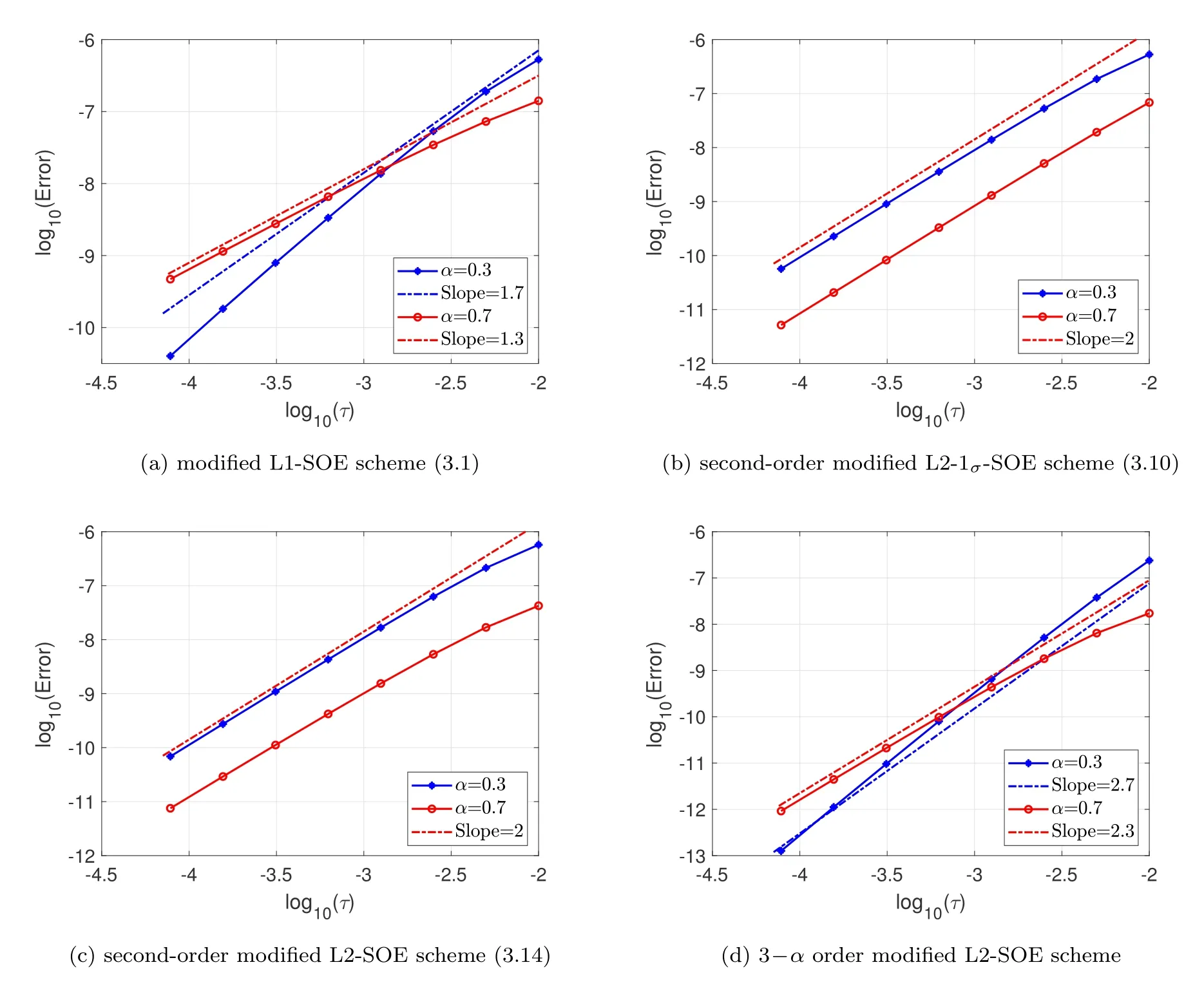
Figure 1: (Example 4.1): Error versus the time step sizes for the proposed schemes with ε2=0.1,T=0.1,and α=0.3,0.7.

In Fig.2,the errors of the proposed schemes with respect to the maximum time step sizesτare plotted in log-log scale,respectively.It is observed that the modified L1-SOE scheme(3.1),the second-order modified L2-1σ-SOE scheme(3.10),the secondorder modified L2-SOE scheme(3.14),and the(3-α)-order modified L2-SOE scheme all achieveα-order in time on the uniform temporal mesh,i.e.,r=1,which indicates the initial low regularity of the solution is abouttα.While the optimal high order accuracy of the proposed schemes are all achieved with the optimal graded meshesr=for the modified L1-SOE scheme(3.1),r=for both the modified L2-1σ-SOE scheme(3.10)and L2-SOE scheme(3.14),andr=for the(3-α)-order modified L2-SOE scheme (3.14),respectively.In addition,we plot the error behaviors of theξnandξnV(ξn)with the optimal gridded meshes for these four types of the proposed schemes in Figs.2(e) and (f),respectively.Here,we setV(ξ)=1+sin(1-ξ) for no more than second-order schemes,andV(ξ)=3-3ξ+ξ2for the modified(3-α)-order L2-SOE scheme.It is observed that,although the error behaviors of the numerical solutionξnare only first order in time,the numerical functionsξnV(ξn) achieve second order forV(ξ)=1+sin(1-ξ) and third order forV(ξ)=3-3ξ+ξ2.This indicates that the first-order accuracy ofξnsolved by a first-order method will not affect the corresponding high-order accuracy of the unknown thin film height functionφnby using some proper auxiliary variable functionsV(ξ) satisfying the condition (3.2) or (3.18).

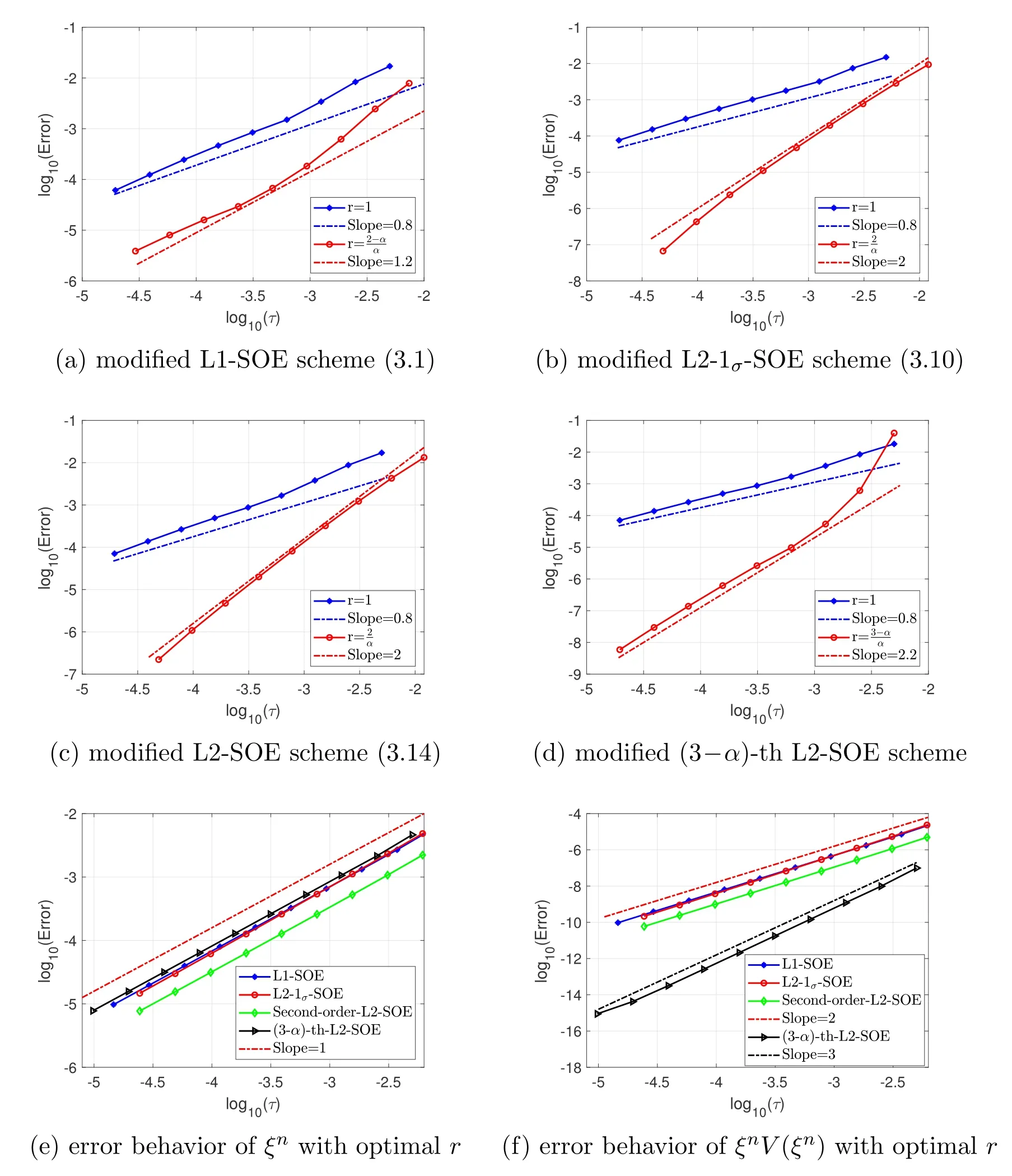
Figure 2: (Example 4.2)Error behaviors of the φn (the first two lines),the ξn and the ξnV(ξn)(the last line) with respect to the time step size for the proposed schemes to the model with α=0.8, ε2=0.01,and T=0.1.

4.2 Coarsening dynamics

To simulate the coarsening dynamics of the time-fractional MBE growth model(1.6),we choose a random initial data ranged from-0.001 to 0.001,and set the width parameterε=0.03.The coarsening dynamics process usually requires a rather long time simulation before reaching its steady state,and the free energy of the model usually undergoes fast and slow change rate stages during this process.Thus robust high-order and unconditionally energy stable numerical schemes are essential important for this simulation to investigate the evolution of thin film epitaxial growth,in which the accuracy of such long-time simulations can be guaranteed,and a timeadaptive strategy can be easily employed to speed up the computation.In this test,the proposed high order schemes are adopted with the following time adaptive strategy based on the energy variation,reported in [38],

where Δtmin,Δtmaxare predetermined minimum and maximum time step sizes,γis a positive constant to be determined.The numerical experiments in the work [38]have shown that using a larger constantγcan improve the accuracy of the numerical solution,but may lead to an increase in the computational cost.However,there is no good criterion for choosing this positive parameterγthat takes into account both the accuracy and efficiency of the numerical schemes with the time adaptive strategy(4.3),and it is usually determined according to numerical experience.In the following tests,we setγ=1e5,as used in[38],for the adaptive simulation of the MBE model.Obviously according to this time adaptive strategy,the numerical scheme will automatically choose small time step sizes in case of large energy variation and big time step sizes while the change rate of the energy is slow,seeing Figs.4 and 7.

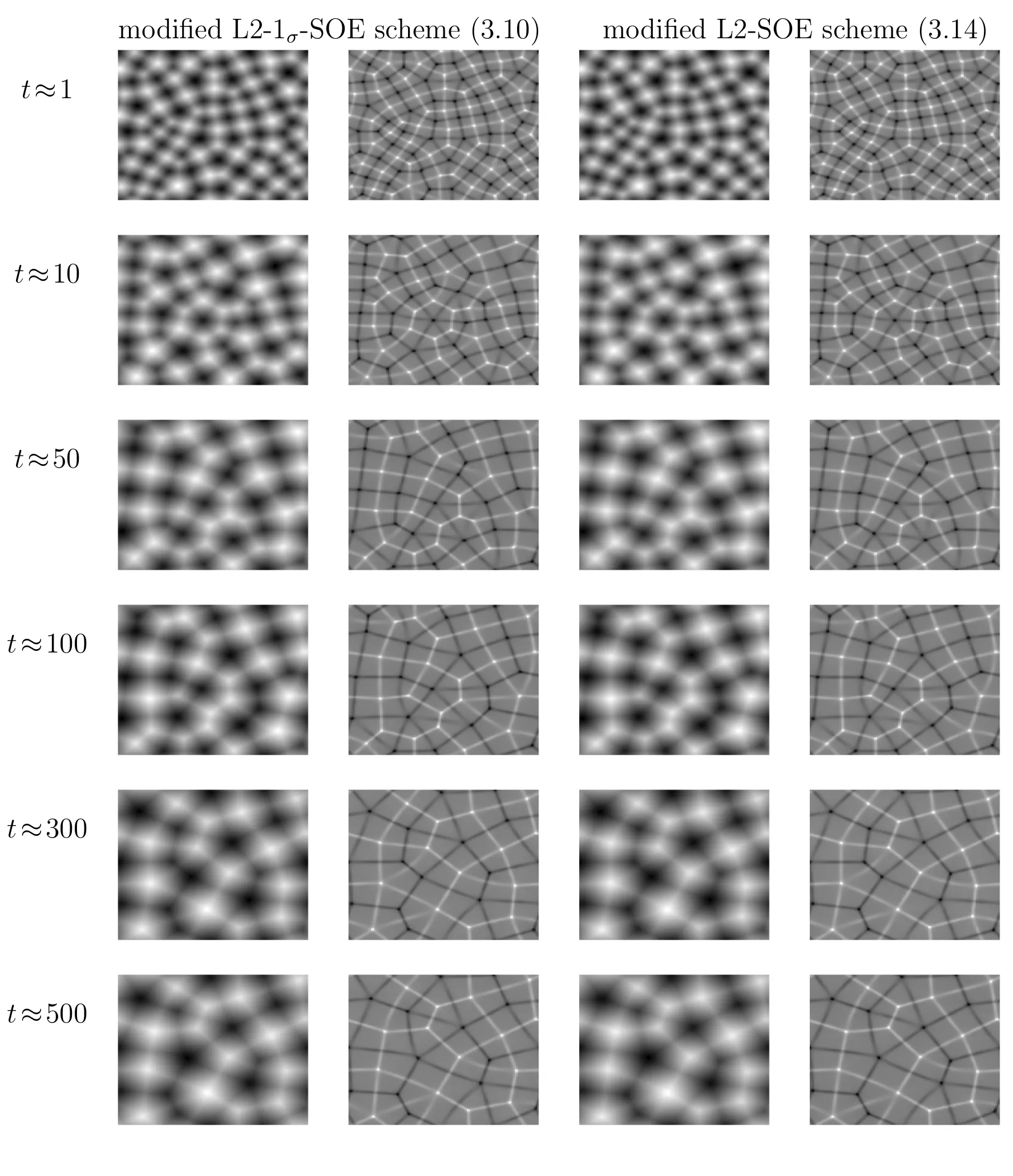
Figure 3: Isolines of the computed height function φ (left) and its Laplacian Δφ (right) for the model(1.6) with α=0.4.

For the 2D time-fractional MBE model (1.6),the computational domain is set to be (0,2π)2,and the simulations are performed by using the modified L2-1σ-SOE scheme(3.10)and the modified L2-SOE scheme(3.14)with 128×128 Fourier modes for spatial discretization,respectively.To deal with the initial low regularity of the solution,we adopt the graded mesh (1.7) with parameterr=andN=1000 in the first subinterval [0,0.1] and the time adaptive strategy (4.3) with Δtmin=1e-5 and Δtmax=1e-2 in the subinterval (0.1,T].In Fig.3,we plot some snapshots of the height functionφand its Laplacian Δφfor the model (1.6) withα=0.4 at serval different times by using both modified L2-1σ-SOE scheme(3.10)and L2-SOE scheme (3.14).It can be observed that there is no distinguishable difference in the numerical solutions up toT=500 for these two tested second-order schemes,which verifies the accuracy of the proposed schemes.The evolutions in time of the energy and the corresponding adaptive step sizes are also plotted in Fig.4 for these proposed two second-order schemes(3.10)and(3.14),to validate their stability and efficiency with the time adaptive strategy (4.3).

Next,we investigate the scaling of the free energyE(φ)and the surface roughnessW(φ)during coarsening by using the modified L2-SOE scheme(3.14)with the same time adaptive parameters as above.The surface roughness functionW(φ)is defined by

whereβ0(α),β(α),R0(α) andR(α) are real functions ofα.Moreover,it holds thatβ(α)～α/3 andR(α)～α/3.Next,we will again numerically verify these scaling laws by the second-order modified L2-SOE scheme (3.14).In Figs.5(a) and (c),we present the evolutions in time of the energyE(φ) and the corresponding surface roughnessW(φ)of the time-fractional MBE model(1.6)in log-log scales for several different order of fractional derivative:α=0.4,0.5,···,0.9 duringt∈[1,500].We use the linear least square fitting approach to numerically compute the scaling parametersβ(α)andR(α).As shown in Figs.5(b)and(d),the energy dissipation rates and the growth rates of the roughness are approximatelyandfor all tested differentα,respectively.Then we again numerically validate the scaling law (4.4),which consists well with the results reported in [7,21].

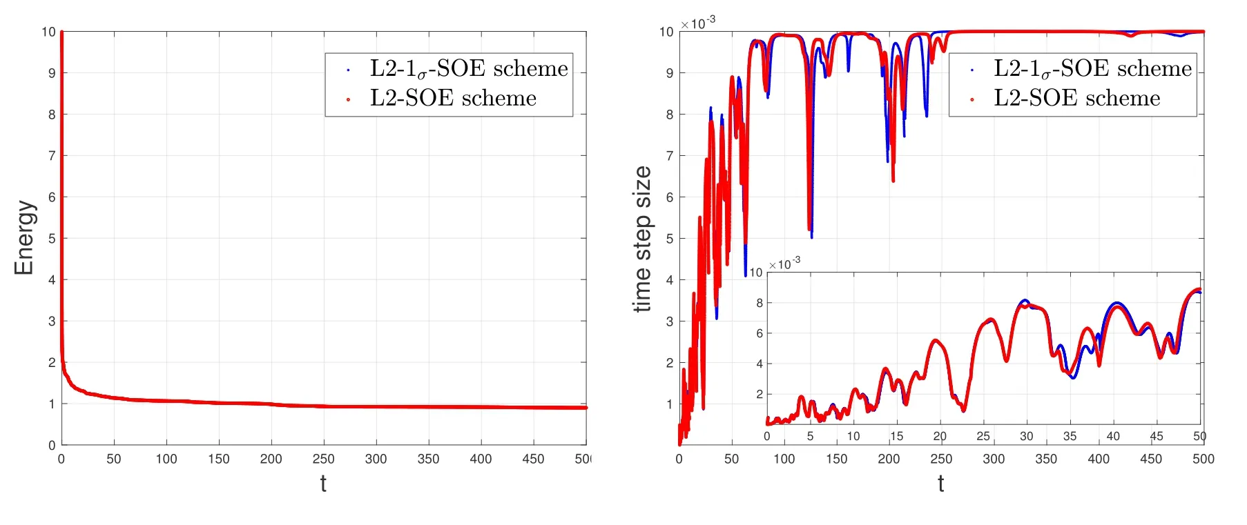
Figure 4: Evolutions in time of the energy (left) and the adaptive time step size (right) for the model(1.6) with α=0.4.

Finally,we show the coarsening dynamics behaviors of the 3D model (1.6) with different time-fractional orderα.The computational domain is set to be(0,2π)3,and a random initial data ranging from-0.001 to 0.001 is used for this test.Simulations are performed by the second-order modified L2-SOE scheme(3.14)with 128×128×128 Fourier modes and the same adaptive time strategy parameters as the case of the above tested 2D model.In Fig.6,we plot several snapshots of iso-surfaces of height functionφ=0 and the density fieldφfor the 3D model (1.6) withα=0.4 andα=0.9,respectively.We observe that the coarsening dynamics of the small time-fractional orderα=0.4 is faster than the one of caseα=0.9 at the early stage.Then the growing speed of the thin film slows down significantly at the later stage when the fractional orderαdecreases.This result consists with the one of 2D case reported in [11,17].The mechanism behind this phenomenon is unclear now and deserves further study in the future.The corresponding evolutions of the computed free energy and the adaptive time step sizes are also displayed in Fig.7.

5 Concluding remarks

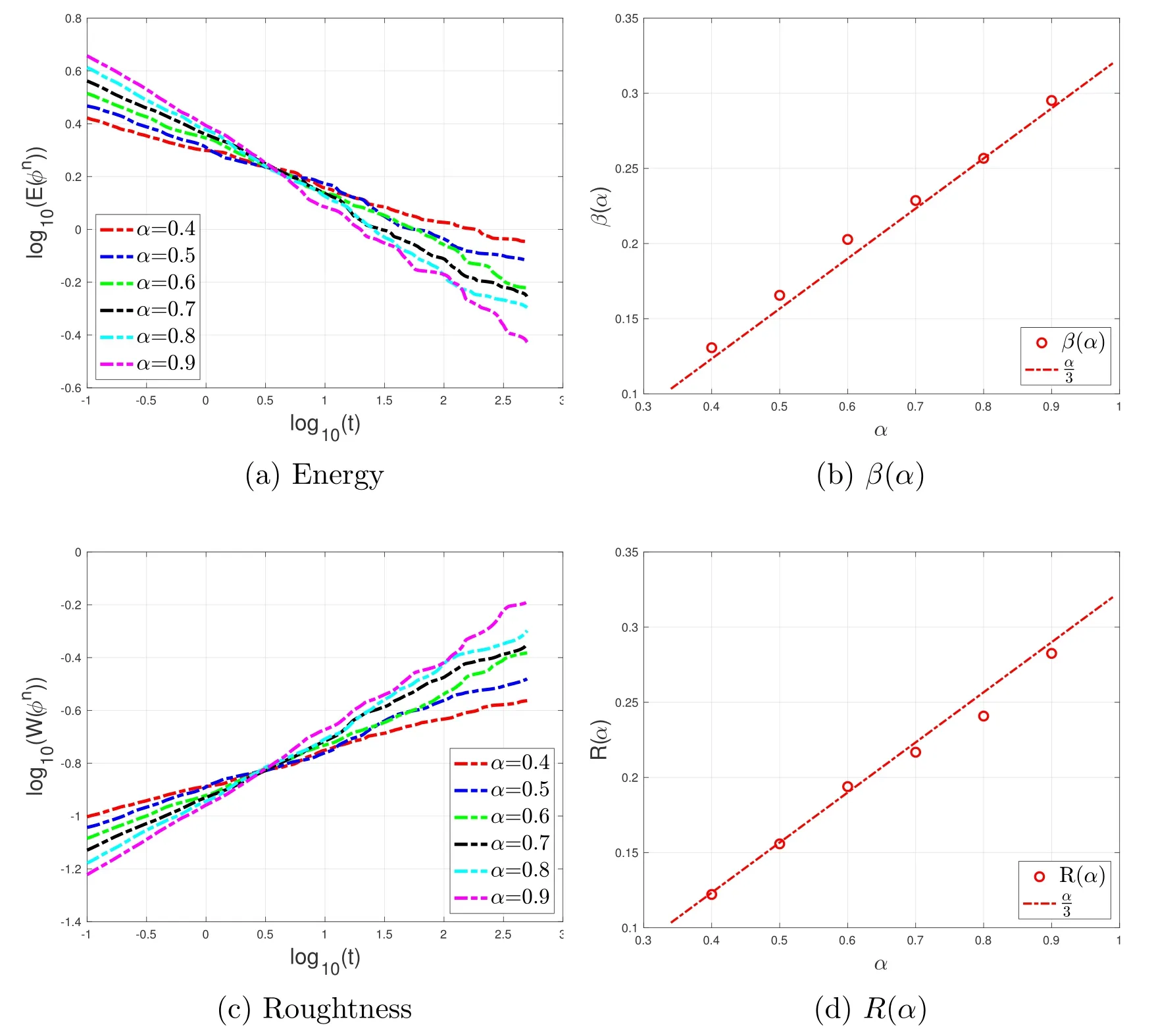
Figure 5: Evolutions of the energy (top) and roughness (bottom) of the MBE growth model (1.6).

We have developed several high-order and nonlocal energy dissipative schemes for the time-fractional MBE growth model,including the fast modified L1-SOE,L2-1σ-SOE,and L2-SOE schemes.The SOE technique is used to discretize the history part of the fractional derivative,which can greatly reduce the amount of computing storage and improve computing efficiency.Furthermore,a scalar auxiliary variable is introduced to deal with the nonlinear term and history part of the fractional derivative,and a first order method is adopted in discretization of the SAV equation.This plays an essential role in derivation of the discrete nonlocal energy dissipation law of the proposed high order schemes.The unconditional nonlocal energy decreasing stabilities of the proposed schemes have been rigorously established on the nonuniform mesh with a mild restriction on the adjacent time-step ratios.Several numerical tests are presented to numerically validate the accuracy and efficiency of the proposed numerical schemes.Due to non-locality of the fractional derivative and complexity of the nonlinear potential function,the corresponding error analysis of the proposed schemes seems to be non-trivial,and requires further investigation.

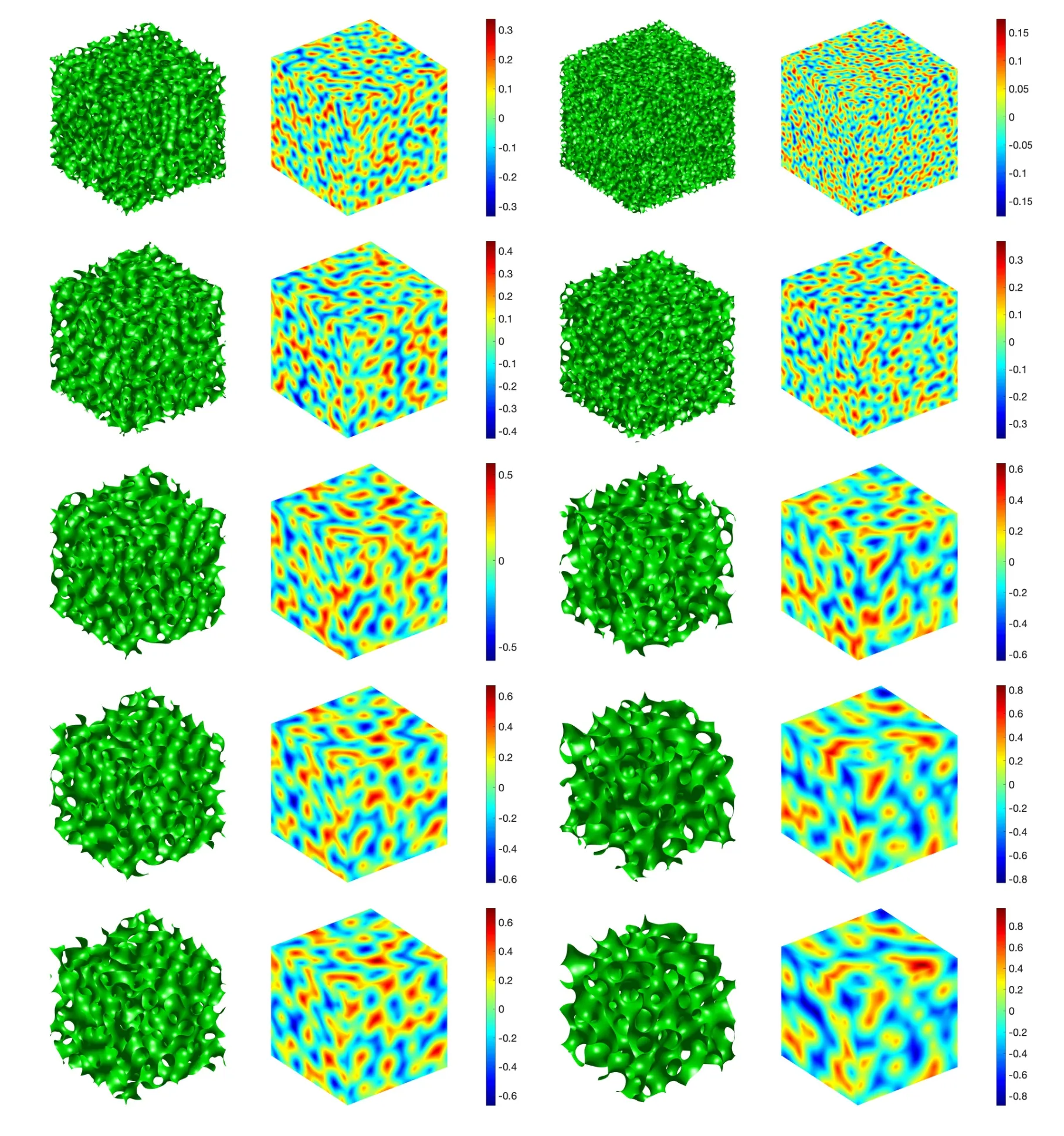
Figure 6: Snapshots of the iso-surfaces of the height function φ=0 (the first and third columns) and density field φ(the second and last columns)for the 3D model(1.6)with α=0.4(the first two columns)and α=0.9 (the last two columns) around the times t=0.1,1,10,30 and 50.

Acknowledgements

D.Hou’s work is partially supported by NSFC grant 12001248,the NSF of Jiangsu Province grant BK20201020,the NSF of Universities in Jiangsu Province of China grant 20KJB110013 and the Hong Kong Polytechnic University grant 1-W00D.Z.Qiao’s work is partially supported by Hong Kong Research Grants Council RFS grant RFS2021-5S03 and GRF grant 15302122,the Hong Kong Polytechnic University grant 1-9BCT,and CAS AMSS-PolyU Joint Laboratory of Applied Mathematics.T.Tang’s work is partially supported by the Guangdong Provincial Key Laboratory of Interdisciplinary Research and Application for Data Science under UIC 2022B1212010006.