Study on Temperature Distribution of Specimens Tested on the Gleeble 3800 at Hot Forming Conditions

Tao Gao, Long Ma, and Xiao-Guo Peng

Study on Temperature Distribution of Specimens Tested on the Gleeble 3800 at Hot Forming Conditions

Tao Gao, Long Ma, and Xiao-Guo Peng

——Taking Ti-6Al-4V specimens into consideration, the coupled thermal-electrical finite element model has been developed in Abaqus/Explicit to simulate the heating process in Gleeble 3800 and to study the temperature history and distribution in the specimen. In order to verify the finite element (FE) results, thermal tests are carried out on Gleeble 3800 for a Ti-6Al-4V specimen with a slot to in the centre of the specimen. The effects of the specimen size, heating rate, and air convection on the temperature distribution over the specimen have been investigated. The conclusions can be drawn as: the temperature gradient of the specimen decreases as the specimen size, heating rate, and vacuuming decrease.

Index Terms——Coupled thermal-electrical simulation, hot forming, thermo-mechanical testing, temperature distribution.

1. Introduction

Gleeble 3800 is a physical material simulation system, which is widely used to investigate viscoplastic deformation and microstructural evolution phenomena of materials in hot metal forming conditions[1]-[5]. Resistance heating is used in Gleeble to achieve rapid heating and cooling in specimens. However, during a hot compression test there exists a non-uniform temperature distribution in the specimen due to the difference of the electrical conductivities of the specimen and anvils, air convection and radiation of the specimen, and heat transfer between anvils and the specimen. The non-uniform temperature distribution in the specimen may directly affect the accuracy of test results. Therefore, it is necessary to studythe temperature distribution of specimens tested on the Gleeble thermo-mechanical simulator.

Research on this above problem, however, was exceedingly limited. Brownet al.[6]investigated the thermal behavior of specimens in a Gleeble material simulator using a finite difference method. Numerical temperature predictions have been compared with experimental temperature measurements performed on 2024 aluminium alloy, 0.2% plain carbon steel, and 316 austenitic stainless steel specimens in the simulator. Norriset al.[7]developed a three-dimensional, explicit finite difference model to simulate the thermal behaviour of Gleeble thermomechanical simulator specimens.

Finite element method (FEM) has become an alternative approach to accurately calculate the temperature history and distribution with complicated boundary conditions. In this paper, taking Ti-6Al-4V specimens into consideration, the coupled thermal-electrical finite element method has been developed in Abaqus/Explicit to simulate the heating process in Gleeble 3800 and to study the temperature history and distribution in the specimen. In order to verify the FE modeling results, thermal tests were carried out on Gleeble for a Ti-6Al-4V specimen with a slot to the centre of the specimen. The effects of specimen size, heating rate, and air convection on the temperature distribution over the specimen have been investigated numerically. The obtained results provide a significant basis for optimizing test programs, so that accurate testing results can be obtained from Gleeble.

2. Methodology of Thermal Electrical FE Analysis

Coupled thermal-electrical analyses are conducted by using a commercial finite element analysis software (Abaqus ver. 6.10-1). For the first step of the analysis, the electrical potential of a specimen exposed to a concentrated electrical current attributable to a lightning strike is calculated under a given electrical boundary condition. Successively, the transient heat transfer analysis is conducted by the application of Joule heat generation to each finite element under a given thermal boundary condition. The temperature dependency of electrical conductivity is adopted for the analysis as described later, therefore the electrical and thermal analyses are fully coupled. The theoretical background for the calculation isbriefly summarized as follows[8].

The equation of conservation of charge is as shown

wherevis any control volume of which surface isS,nis the outward normal toS,Jis the electrical current density (current per unit area), andrcis the internal volumetric current source per unit volume.

Using this definition of the electrical field, Ohm’s law can be written as shown below

whereφ,E, andσrespectively signify the electrical potential field, electrical potential, and electrical conductivity. The constitutive relation is linear; it assumes that the electrical conductivity is independent of the electrical field. A basic equation for electrical analysis is obtained by introducing Ohm’s law (2) to “weak form” of the conservation of charge equation

whereis electrical current density towards a control volume. Joule’s law describes the rate of electrical energy,Pec, dissipated by current flowing through a conductor, as in the following equation:

On the other hand, a basic equation for thermal conductive analysis is as follows:

whereθ,k,ρ,Cv,q, andrrespectively signify the temperature, thermal conductivity, density, specific heat, heat flux density towards a control volumev, and the heat generation density.

For the coupled thermal-electrical analysis, the steady-state electrical analysis and transient thermal analysis are sequentially conducted in each time increment. As a result, the electrical potential, electrical current, Joule heat generation, temperature of each element can be obtained. Temperature dependent material properties are updated after the calculation of each time increment.

3. FE Modeling of Heating Process in Gleeble 3800

3.1 FE Model

In a Gleeble simulator, a cylinder of Ti-6Al-4V specimen with a height of 15 mm and a diameter of 10 mm is used. Four cylinders with a height of 6 mm and a diameter of 20 mm constitute the anvil. Graphite sheets are used for lubricating the specimen and the anvil, and the thickness of graphite sheets is 0.30 mm. Resistance heating is used in the Gleeble to achieve a rapid heating and cooling in specimens. The coupled thermal-electrical finite element method has been developed in Abaqus/Explicit to simulate the heating process in Gleeble 3800. Due to symmetry with respect to the midplane, only a quarter of the axisymmetric specimen was modeled using the 2D coupled thermal-electrical elements as shown in Fig. 1. Due to the water cooling, the temperature of the end of anvil 4 is assumed as 50°C.

Fig. 1. 2D FEM model of the heating process in Gleeble 3800.

The values of physical parameters of Ti-6Al-4V are obtained from [9]. The density, the specific heat, and the Joule heat fraction are 4440 kg/m3, 3830 J/(kg·°C), and 1, respectively. The temperature-dependent thermal conductivities are shown in Table 1. The temperaturedependent electrical conductivities are shown in Table 2.

The material of the anvils is tungsten steel and the values of physical parameters are obtained from [9]. The density, specific heat, Joule heat fraction, thermal conductivity, and electrical conductivity are 1440 kg/m3, 813 J/(kg·°C), 1, 16 W/(m·°C), and 1380000 ?-1·m-1, respectively.

Table 1: Temperature-dependent thermal conductivities of Ti-6Al-4V

Table 2: Temperature-dependent electrical conductivities of Ti-6Al-4V

The values of physical parameters of graphite are obtained from [9]. The density, specific heat, Joule heat fraction, thermal conductivity, and electrical conductivity are 2200 kg/m3, 710 J/(kg·°C) and 1, 1950 W/(m·°C), and 105 ?-1·m-1, respectively.

3.2 Boundary Conditions and Loads

All parts are assumed to contact firmly, so the clearance is selected as 0, and the gap electrical conductance is a very large value. The gap conductance is obtained from [10] as 104 W/(m2·°C).

While there is air in the chamber of a Gleeble simulator, the air convection coefficient is 20 W/(m2·°C). The radiation emissivity is 0.5.

A typical heating cycle is selected to simulate the heating process as shown in Fig. 2. It consists of three processes. The first process is the rapid heating process with the heating rate 20°C/s and the temperature of the specimen reaches 880 °C in 44 s. The following process is the slower heating process with the heating rate 2°C/s and the temperature of the specimen rises from 880 °C to 920°C in 20 s. The last process is the soaking process and the specimen is kept at 920°C. The electrical potential is applied in the coupled thermal-electrical analysis. The magnitude of the electrical potential can be controlled by the temperature of point A in Fig. 1.

Fig. 2. Typical heat cycle in a Gleeble material simulator.

3.3 Verification

In order to verify the FE modeling results, thermal tests are carried out on Gleeble for a Ti-6Al-4V specimen with a slot to the centre of the specimen. The tested specimen is shown in Fig. 3.

Fig. 3. Photographs of specimen: (a) a Ti-6Al-4V specimen with a slot to the central of the testpiece and (b) the specimen having thermal couples embedded.

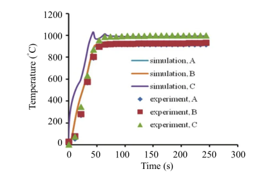
Fig. 4. Comparison of temperature of points (A, B and C) between simulation and experiments.

The locations of measure points (A, B and C) used to study the temperature distribution are shown in Fig. 1. The comparisons of temperature distributions of measured points from FE simulation with those from experiments are shown in Fig. 4. It can be seen that the FE results are in good agreement with experimental ones. This shows that the model proposed in this paper is practicable and reliable, which provides an effective method to study the temperature history and distribution in the specimen and to investigate the effect of specimen size, heating rate, and air conditions on the temperature distribution over the specimen.

4. Results and Discussion

4.1 Study of the Temperature History and Distribution in the Specimen

The heating processes are simulated and analyzed by using the coupled thermal-electrical finite element method. In order to effectively analyze the temperature distribution over the specimen, the middle time and the end time of each process are selected, i.e. 22 s, 44 s, 54 s, 64 s, 100 s, and 244 s. The temperature distributions of the specimen under the different time are shown in Fig. 5. It can be clearly seen that the temperature of the specimen end closed with graphite is the highest during the whole heating and soaking process. The reason is that both the thermal conductivity and the electrical conductivity of graphite are larger, and its temperature increases at a higher rate with regards to the same electrical current. From this figure we can also see that the gradient of temperature distribution of the specimen increases with the heating time during the rapid heating process, and then decreases gradually during the following two processes. The difference of the temperature over the specimen can reaches over 153°C at the end of the rapid process, 92°C at the end of the slower heating process, and 70°C at the end of soaking process, respectively. The peak temperature is 1027°C at the end of the rapid heating process, and then 1013°C at the end of the slower heating process. So the temperatures distributions at the end of both the rapid and the slower heating under different parameters are adopted at the following analyses.

Fig. 5. Temperature distribution of the specimen at different times: (a) 22 s, (b) 44 s, (c) 54 s, (d) 64 s, (e) 100 s, and (f) 244 s.

4.2 Effects of Specimen Size on Temperature Distribution

The temperature distributions of this specimen at the end of both the rapid and slower heating processes are shown in Fig. 6 by changing the specimen size to a height of 12 mm and a diameter of 8 mm. Comparing Fig. 5 and Fig. 6, it can be seen that the gradient of temperature distribution of the specimen decreases with the decreasing of the specimen size. The max of the temperature of the specimen decreases from 1027°C to 991°C.

Fig. 6. Temperature distribution of the specimen with as a height of 12 mm and a diameter of 8 mm at: (a) the end of the rapid heating process and (d) the end of the slower heating process.

4.3 Effects of Heating Rate on Temperature Distribution

Keeping the parameters at Section 4.2, both the rapid and slower heat rates are selected 10°C/s and 1°C/s, respectively. The temperature distributions under this heating rate are shown in Fig. 7. Comparing Fig. 6 and Fig. 7, it can be concluded that the gradient of temperature distribution of the specimen decreases with the decreasing of the heating rate. The max of the temperature of the specimen decreases from 991°C to 980°C.

Fig. 7. Temperature distribution of the specimen at: (a) the end of the rapid heating process with the heat rates 10°C/s and (d) the end of the slower heating process with the heat rates 1°C/s .

4.4 Effects of Air Condition on Temperature Distribution

Based on the condition at Section 4.3, by vacuuming the chamber, the temperature distributions of the specimen are shown in Fig. 8. It is clear that the gradient of temperature distribution of the specimen decreases with vacuuming. The max of the temperature of the specimen decreases from 980°C to 964°C.

Fig. 8. Temperature distribution of the specimen with vacuuming at: (a) the end of the rapid heating process and (d) the end of the slower heating process.

5. Conclusions

A coupled thermal-electrical FEM model corresponding to reality has been proposed for a heating process in Gleeble 3800. The temperature history and distribution has been studied, and the effects of specimen size, heating rate, and air conditions on the temperature distribution over the specimen have been investigated. The conclusions can be drawn that the gradient of temperature distribution decreases as the specimen size, the heating rate, and the vacuuming decrease.

Acknowledgment

The authors gratefully acknowledge the provision of computing and testing facilities and its support by Mechanics and Materials Division, Department of Mechanical Engineering, Imperial College London.

[1] J. Lin and T. A. Dean, “Modeling of microstructure evolution in hot forming using unified constitutive equations,”Journal of Materials Processing Technology, vol. 167, pp. 354-362, Aug. 2005.

[2] J. Luo, M. Li, X. Li, and Y. Shi, “Constitutive model for high temperature deformation of titanium alloy using internal state variable,”Mechanics of Materials, vol. 42, pp. 157-165, Feb. 2010.

[3] X.-G. Fan and H. Yang, “Internal-state-variable based self-consistent constitutive modeling for hot working of two-phase titanium alloys coupling microstructure evolution,”Int. Journal of Plasticity, vol. 27, pp. 1833-1852, Nov. 2011.

[4] M. A. J. Taleghani, E. M. R. Navas, M. Salehi, and J. M. Torralba, “Hot deformation behavior and flow stress prediction of 7075 aluminium alloy powder compacts during compression at elevated temperatures,”Materials Science and Engineering: A, vol. 534, pp. 624-631, Feb. 2012.

[5] Q. Bai, J. Lin, T. A. Dean, D. S. Balint, T. Gao, and Z. Zhang,“Modeling of dominant softening mechanisms for Ti-6Al-4V in steady state hot forming conditions,”Materials Science and Engineering: A, vol. 559, pp. 352-358, Jan. 2013.

[6] S. G. R. Brown, J. D. James, and J. A. Spittle, “A 3D numerical model of the temperature-time characteristics of specimens tested on the Gleeble thermomechanical simulator,”Modeling Silul. Mater. Sci. Eng., vol. 5, pp. 539-548, Jul. 1997.

[7] S. D. Norris and I. Wilson, “Application of 3D numerical modeling for thermal profile optimization on the Gleeble thermomechanical simulator,”Modeling Silul. Mater. Sci. Eng., vol. 7, pp. 297-309, Feb. 1999.

[8]Abaqus Analysis User’s Manual, 6.7.2, Coupled Thermal-Electrical Analysis, Dassault Systems Simulia, 2010.

[9] X.-F. Lu,China Materials Engineering Canon, Beijing: Chemical Industry Press, 2006, pp. 585.

[10] H.-T. Ding, N.-G. Shen, and Y.-C. Shi, “Thermal and mechanical modeling analysis of laser-assisted micro-milling of difficult-to-machine alloys,”Journal of Materials Processing Technology, vol. 212, pp. 601-613, Mar. 2012.

Tao Gao was born in Hubei, China in 1979. He received the Ph.D. degree in material processing engineering from the Northwestern Polytechnical University, Xi’an in 2008. He is an associate professor with the School of Mechanical, Electronic and Industrial Engineering, University of Electronic Science and Technology of China (UESTC). His research interests include CAD modeling and FE analysis of metal forming process, and optimal design methods.

Long Ma was born in Jilin, China in 1988. He received the B.S. degree in electrical engineering from UESTC, Chengdu in 2011. He is currently pursuing the M.S. degree with the School of Mechatronics Engineering, UESTC. His research interests include material modeling and mechanical structure design.

Peng-Xiao Guo was born in Sichuan, China in 1989. He received the B.S. degree from Wuhan Institute of Technology, Wuhan in 2012. He is currently pursuing the M.S. degree with UESTC. His research interests include digital design and simulation and materials machining.

Manuscript received October, 2013; revised February 17, 2014. This work was supported by the Fundamental Research Funds for the Central Universities of China under Grant No. A03007023801073.

T. Gao is with the School of Mechanical, Electronic and Industrial Engineering, University of Electronic Science and Technology of China, Chengdu 611731, China (Corresponding author e-mail: gaotao@uestc.edu.cn).

L. Ma and X.-G. Peng are with the School of Mechanical, Electronic and Industrial Engineering, University of Electronic Science and Technology of China, Chengdu 611731, China (e-mail: malonguestc@163.com; Peng35233hot@163.com).

Color versions of one or more of the figures in this paper are available online at http://www.journal.uestc.edu.cn.

Digital Object Identifier 10.3969/j.issn.1674-862X.2014.04.015