
Large-eddy simulation of shock-wave/turbulent boundary layer interaction with and without SparkJet control
2016-11-23 06:10YngGungYoYufengFngJinGnTinLiQiushiLuLipeng
CHINESE JOURNAL OF AERONAUTICS 2016年3期
Yng Gung,Yo Yufeng,Fng Jin,c,*,Gn Tin,Li Qiushi,Lu Lipeng
aNational Key Laboratory of Science and Technology on Aero-Engine Aero-Thermodynamics,School of Energy and Power Engineering,Beihang University,Beijing 100083,China
bFaculty of Environment and Technology,University of the West of England,Bristol BS16 1QY,United Kingdom
cComputer Science and Engineering Department,Scienceamp;Technology Facilities Council(STFC),Daresbury Laboratory,Warrington WA4 4AD,UK
Large-eddy simulation of shock-wave/turbulent boundary layer interaction with and without SparkJet control
Yang Guanga,Yao Yufengb,Fang Jiana,c,*,Gan Tiana,Li Qiushia,Lu Lipenga
aNational Key Laboratory of Science and Technology on Aero-Engine Aero-Thermodynamics,School of Energy and Power Engineering,Beihang University,Beijing 100083,China
bFaculty of Environment and Technology,University of the West of England,Bristol BS16 1QY,United Kingdom
cComputer Science and Engineering Department,Scienceamp;Technology Facilities Council(STFC),Daresbury Laboratory,Warrington WA4 4AD,UK
The efficiency and mechanism of an active control device''SparkJetquot;and its application in shock-induced separation control are studied using large-eddy simulation in this paper.The base flow is the interaction of an oblique shock-wave generated by 8°wedge and a spatially-developing Ma=2.3 turbulent boundary layer.The Reynolds number based on the incoming flow property and the boundary layer displacement thickness at the impinging point without shock-wave is 20000.The detailed numerical approaches were presented.The in flow turbulence was generated using the digital filter method to avoid artificial temporal or streamwise periodicity.The numerical results including velocity pro file,Reynolds stress pro file,skin friction,and wall pressure were systematically validated against the available wind tunnel particle image velocimetry(PIV)measurements of the same flow condition.Further study on the control of flow separation due to the strong shock-viscous interaction using an active control actuator''SparkJetquot;was conducted.The single-pulsed characteristic of the device was obtained and compared with the experiment.Both instantaneous and time-averaged flow fields have shown that the jet flow issuing from the actuator cavity enhances the flow mixing inside the boundary layer,making the boundary layer more resistant to flow separation.Skin friction coefficient distribution shows that the separation bubble length is reduced by about 35%with control exerted.
1.Introduction
Shock-wave/turbulent boundary layer interaction(SWTBLI)happens ubiquitously in high-speed vehicles,including transonic airfoils,supersonic inlets,control surfaces of aircrafts,missile base flows,reaction control jets,and over expanded nozzles.Among these configurations,maximum mean and fluctuating wall pressure and thermal loads are often found in the vicinity of SWTBLI region and have great influences on the high-speed flying vehicles and their component geometry designs,material selections,fatigue life,thermal production system designs,weight and cost.1Over the past sixty years since the SWTBLI phenomenon was firstly observed by Ferri,2a large number of configurations have been investigated over a wide range of flow conditions.Although substantial databases of experimental3and theoretical4results have been accumulated,the underlying physical flow phenomenon is still not fully understood yet and remains one major subject of active investigation due to its great practical importance and extreme complexity,which hindered the establishment of an effective and applicable turbulence model for such flow.5Some extensive reviews on the achievements and remaining challenges were given previously by Green6,Adamson and Messiter,7Delery,8Dolling1and most recently by Knight9as well as Babinsky,10–12etc.
With the rapid increase of computing power in recent decades,especially the fast development of high-performance computing(HPC)platforms,modern computational fluid dynamics(CFD)technique is now playing a much more important role in aerodynamic researches.In particular,direct numerical simulation(DNS)and large-eddy simulation(LES)become essential research tools for fundamental in-depth flow mechanism studies.13,14While DNS resolves flow structures of all scales and can get full temporal-spatial information of a turbulent flow field,the computational grid must be fine enough to resolve the Kolmogorov scale thus would be too expensive for relatively high Reynolds number flows.By applying a low-pass filter,LES resolves only large scale structures that dominate the major dynamics of the turbulence and model the unresolved subgrid scales.15Thus the LES grid requirement is much less severe than that of the DNS,which saves computing resources and extends the flow range that can be studied.Nevertheless,LES maintains some major advantages of DNS,namely providing the full spatial and temporal flow information down to the resolved scales.Based on these,LES is increasingly becoming an appropriate tool to study the unsteady complex SWTBLI flows and some noticeable researches have been published in the last two decades.16–18These works have greatly deepened our understanding about the SWTBLI flows.
One of the important problems in SWTBLI is that the strong adverse pressure gradient due to the shock-wave can trigger large-scale flow separation,resulting in significant total pressure loss and flow distortion.Furthermore,the lowfrequency unsteadiness of the separation shock-wave motion which can cause severe structural loads/resonances and may eventually lead to fatigue is also thought to be linked with the so-called''breathquot;motion of the separation zone.19Hence,controlling the shock-wave induced flow separation is always a focus in SWTBLI researches and many active and passive control approaches have been proposed.20Passive control devices include vortex generators21–23,Mesoflaps24–26ventilation duct or porous wall over cavity,27,28etc.Active controls using plasma are now gaining more and more attentions in high speed flows for their advantages of avoiding any ad hoc mechanical components,enabling high effectiveness and ability of high-frequency modulation.The primary mechanisms of plasma flow control include electro-hydrodynamic(EHD)control and magneto-hydrodynamic(MHD)control,as well as thermal methods.The SparkJet actuator studied in this paper belongs to the third type.
The SparkJet actuator was originally developed by Land et al.29aiming for high-speed flow control.This actuator can manipulate high-speed flow without introducing additional mechanical components.The SparkJet is a zero net mass flow(ZNMF)device that consists of a small chamber with electrodes inside and a discharge orifice.High chamber pressure is generated by rapidly heating the gas inside the chamber using an electrical spark discharge.Then the high pressure gas would be ejected into the main flow field through the orifice,forming a jet stream.Fig.1 shows a single cycle of SparkJet operation which consists of three distinct stages:energy deposition,discharge,and refilling.Fig.2 is the photographical view of a laboratory SparkJet device which is a modified version of Cybyk's original invention,experimentally investigated by Reedy et al.30(the device is axisymmetric and the radial and axial coordinates r and z are shown in the figure).Characteristics of this device have been extensively investigated in experimental studies.31–41Narayanaswamy et al.42,43applied such a device to control the flow separation and low-frequency unsteadiness in a supersonic compression corner flow.
The main purpose of this paper is to investigate the property of SparkJet and the feasibility of its application in SWTBLI separation controls.

Fig.1 Schematic of SparkJet work cycle.

Fig.2 SparkJet device used in experiment of Reedy et al.30
The paper is organized as follows:In Section 2,numerical details are presented,including governing equation,numerical schemes,inflow turbulence generation method and adopted subgrid scale model.In Section 3,numerical results of the SWTBLI base flow are presented and validated by comparing with the experimental measurements of the same flow condition conducted by the research team at Institut Universitaire des Systèmes Thermiques Industriels(IUSTI)in Marseille,France.In Section 4,the setup of SparkJet in LES modeling is described and the generated jet is validated against the experiment of Reedy et al.41The single-pulsed characteristics of the flow with the SparkJet control are then further analyzed.Finally,some conclusions are given in Section 5.
2.Numerical approach
2.1.Governing equation
The numerical approach adopted in this paper is LES due to its advantages mentioned in the introduction.The conceptual idea of LES is to fully resolve the large-scale energycontaining turbulence structures and only model the effect of the unresolved smaller scales of turbulent flow.The spatialscale separation is represented by the convolution product defined in Eq.(1):

where q is an arbitrary variable,qˉthe filtered variable,G the filter convolution kernel,andΔˉits associated characteristic cutoff length scale,x and z are spatial coordinates.The kernel function G satisfies

In compressible flow researches,the following Favre average is a commonly used technique to take account of the effect of density variety.

Applying the above filter and Favre average operator to the Navier–Stokes equations and after some algebraic manipulation,the complete form of the grid-filtered dimensionless compressible Navier–Stokes equations can be written as

The resolved equation of state,the resolved total energy/pressure relation and the resolved viscous shear-stress relations are

The resolved dynamic viscosity is determined by Sutherland's law

where TS=110.4 K and T0=145.77 K according to the present experimental condition.

The subgrid-scale(SGS)terms in the right-hand side of the Eqs.(5)and(6)are
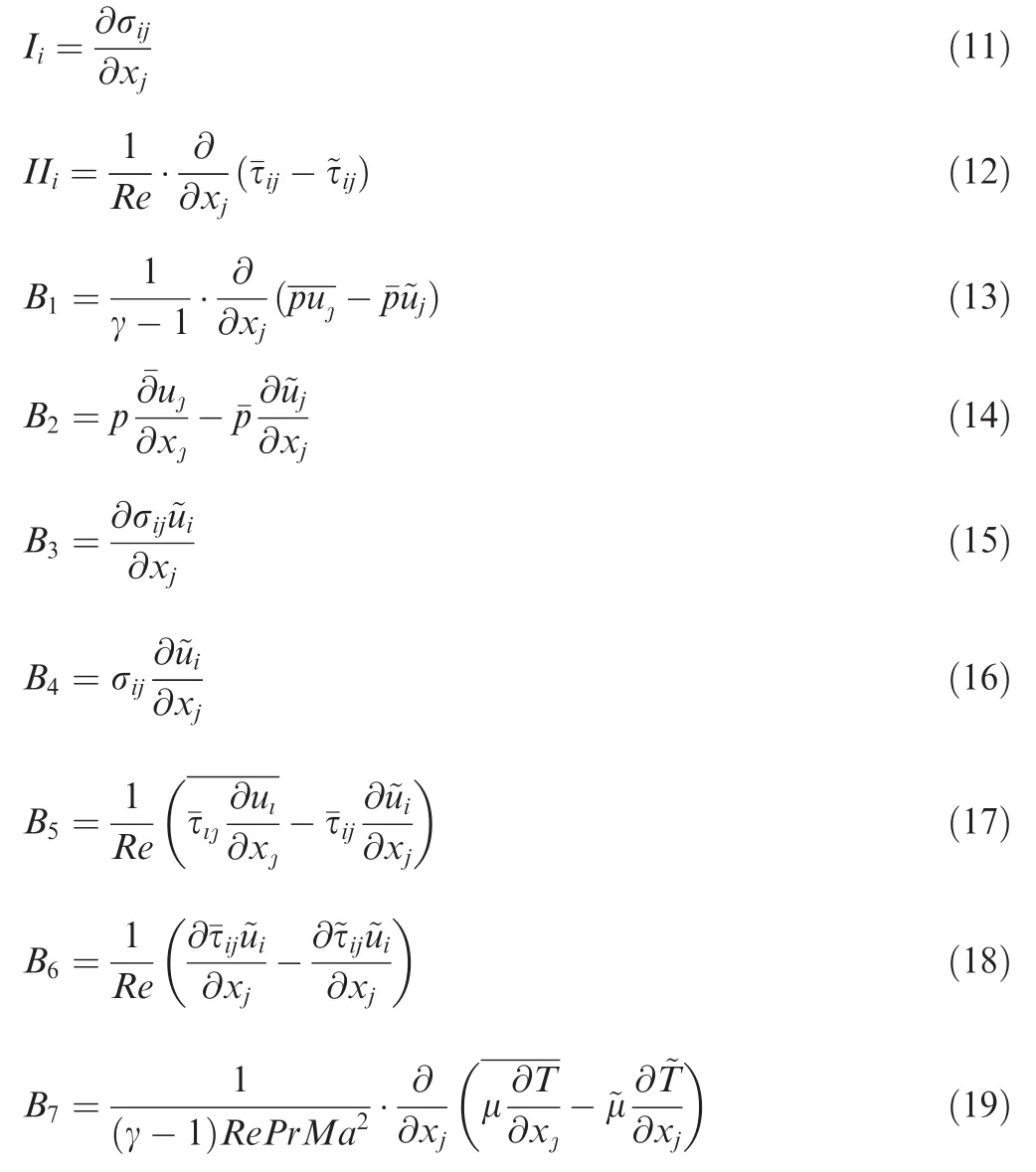
where σijis the SGS stress tensor and defined as

Vreman44looked at all the above SGS terms by analyzing DNS database of a plane compressible mixing-layer at Mach numbers 0.2 and 0.6.He categorized the SGS terms as shown in Table 1.Although the classification was performed for lower Reynolds number and Mach number flows other thanthe high-speed high-Reynolds number flow considered in the present SWTBLI study,the classification is still widely accepted and valid,and has been successfully used in other earlier LES studies of SWTBLI.16–18

Table 1 Classification of SGS terms.
After some mathematical manipulations,the sum of B1and B2can be decomposed into two terms as follows:


The present LES only solves the approximate form of the aforementioned filtered Navier–Stokes equations where terms IIi,B5,B6,B7and D are neglected44and only the SGS stress tensor and the SGS heat flux are modeled.
The SGS stress tensor is modeled via the classical eddyviscosity approach as follows:

where νtis the eddy viscosity andthe deviatory part of the strain-rate tensor computed from the filtered velocity field:

The SGS model used in the present simulation is the mixedtime-scale(MTS)model by Inagaki et al.45The MTS model is essentially based on a dimensionally-consistent physical argument relating to the asymptotic behavior of the eddy viscosity as one approaches the wall and the potential flow.Similar to the widely used dynamic S magrinsky model,the MTS model makes use of a test filter.The eddy viscosity νtis modeled as

where

The constants CMand CTwere originally set to be 0.05 and 10,respectively,by Inagaki et al.45based on a priori test of channel and backward-facing step flow data.However,in the currentimplementation of the model,we have used CM=0.03 and CT=10 based on the application of present LES solver to the compressible turbulent channel flow of Li.46
Once the eddy-viscosity value is obtained,the SGS heat flux is modeled as
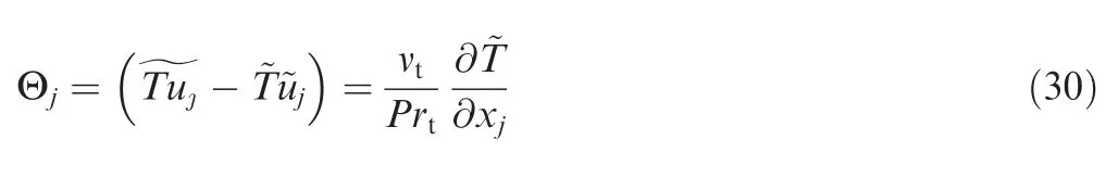
The SGS turbulent Prandtl number Prtwas set as a constant Prt=1.0 in the present simulation,invoking the strong Reynolds analogy(SRA).
2.2.Numerical schemes
The above equations are solved using an in-house high order finite-difference code SBLI.The code employs a fourth-order central difference scheme to calculate derivatives at internal points.Close to boundaries,a stable boundary treatment proposed by Carpenter et al.47is applied,giving the overall fourth order accuracy.Time integration is based on a third-order compact storage Runge–Kutta method.48
For LES of turbulent flow,the longtime integration can accumulate the numerical error and cause the instability of the solution.As proposed by Yee et al.49,the application of the energy estimation method to the Euler equations can be extended to the Navier–Stokes equations in order to stabilize the solution of long time integration problems.Based on this idea,Sandham et al.50applied an entropy splitting approach to calculate the nonlinear terms.The basic procedure consists of a transformation of the equations in a symmetric form using an''entropy variablequot;W,which is introduced as W= ?η/?U,where η = ρξ(S)is an entropy function and ξ(S)is an arbitrary but differentiable function of a dimensionless physical entropy S,S=ln(pρ-γ).The choice of ξ(S)is restricted by a homogeneity requirement and a positive definite condition on the matrix UW= ?U/?W,which can be satisfied by defining ξ(S)=KeS/(α+γ),where K and α are constants.Then the convective terms are split into a conservative portion and a non-conservative portion by a splitting parameter β,both in symmetric form.Finally,the summation by parts propriety can be applied to each portion in order to estimate an upper bound to the energy growth.This will guarantee the stability of the algorithm.The details of entropy splitting method can be found in Ref.50.
A total variance diminishing(TVD)shock capturing scheme and the artificial compression method(ACM)of Yee et al.,49coupled with the Ducros sensor51,are implemented in the code to handle shock-waves and contact discontinuities.The code is made parallel using the message passing interface(MPI)library.A multi-block version of the code was extensively validated by Yao et al.52
As for the boundary condition,periodic boundary conditions are used in the span wise direction.At the wall,the noslip condition is enforced.Furthermore,the wall is considered isothermal with a temperature close to the upstream adiabatic value(assuming a recovery factor of 1).The top(free-stream)and outflow boundaries make use of the characteristic nonreflecting boundary condition53in order to minimize unwanted reflections from the computational-box boundaries.The oblique shock-wave is introduced at the top boundary using the Rankine-Hugoniot relationships.As for the turbulent inflow condition,the generation of inflow turbulent fluctuation is a major issue for LES and DNS computation.In the present simulation,the turbulent inflow turbulence is generated using a digital filter method which will be described in the next section.
2.3.Inflow turbulence generation
The digital filter method incorporates the turbulence first order and second-order moments information with filtered random datasets to generate an artificial inflow condition which prescribes both the real-turbulence Reynolds stress and energy spectra.It has been applied to a series of high speed boundary layer flows54,55due to its advantages of easy-to-implement,short transition distance and introducing no artificial periodicity.Using this method,the velocity at the inflow plane is written as

where Rijis the prescribed Reynolds stress tensor,and Fi(y,z)the filtered independent random variable with the Gaussian distribution updated every time step using the formula:

where Δt is the time step,and τ the Lagrangian timescalein the present implementation,where Ixandare the prescribed inlet mean streamwise velocity and integral length scale,respectively).Thein the above formula are given as

where vl(j,k)are pure Gaussian distributed random numbers,and bjkdigital filter coefficients.The detailed determination method of these coefficients can befound in Ref.56The parameters used to generate the digital filter coefficients are given in Table 2.
The temperature and density fluctuations are then related to the streamwise velocity fluctuation via the formulas below,as implied by SRA.

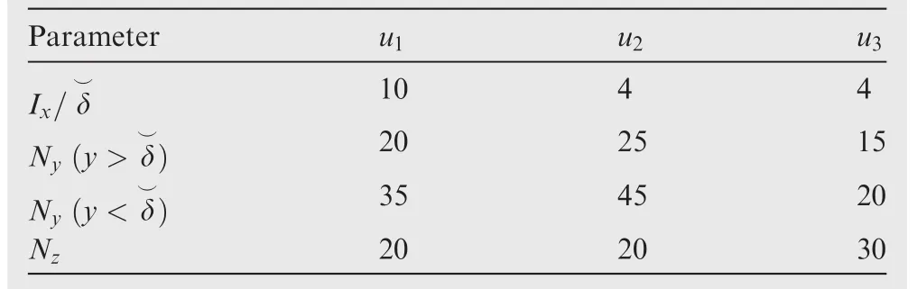
Table 2 Digital filter parameters.
3.SWTBLI results
As mentioned before,the simulation flow condition is consistent with the experiment performed by Dupont et al.57of IUSTI,i.e.,an oblique shock-wave generated by an 8°wedge impinging onto a Mach 2.3 turbulent boundary layer(Note that for all the figure legends in this section,''LESquot;means present LES,and''PIVquot;means PIV measurements of Dupont et al.52,unless otherwise stated).The flow parameters are listed in Table 3.The Reynolds number is based on the boundary layer displacement thickness at interaction point without shock-wave impinging.This flow condition has been previously studied by Garnier et al.16and Touber and Sandham,55also using LES.
In the present simulation,the computation domain is(Lx,Ly,Lz)=(256 mm,51 mm,59 mm),along the streamwise,wall-normal and span wise directions,respectively.For the convenience of comparing with the experimental data,the streamwise domain range is[148,404]mm,which is the same with the physical domain in the experiment.The shock-wave impinging point is at x=336 mm in absence of shock-wave.The grid number in each direction is(Nx,Ny,Nz)=(451,151,281),uniform in the streamwise and the span wise directions while stretched in the wall normal direction.The corresponding grid resolution in each direction is estimated as(Δx+,Δy+,Δz+)=(33,1.3,12),which satisfies the general LES requirement.15
In Fig.3,the impinging shock-wave,reflected shock-wave and expansion fan can be clearly recognized in the time averaged density field.The white dashed line is the average sonic line and the black solid line is the contour line of u=0 that marks the average separation bubble boundary.The mean velocity profile of the equilibrium boundary layer at x=260 mm is validated in Fig.4.Fig.4(a)shows that current LES results are in a good agreement with the data from the PIV measurement,the superscript''*quot;means in dimensional form,and the van-Driest transformed velocity profilein the wall unit in Fig.4(b)agrees well with the classic law of the wall.This testifies that the boundary layer in the upstream of the interaction zone is indeed fully developed.Fig.5 showsthe root mean squared(RMS)Reynolds stress profiles at the same location.LES prediction still agrees well with the particle image velocimetry(PIV)data,except for the near wall region,where the accuracy of PIV measurement may be degraded somehow.The above results have shown that in the region of equilibrium turbulent boundary layer ahead of shock wave impinging location,the present LES results agree well with the available test data.

Table 3 Flow parameters.

Fig.3 Time average density field.

Fig.4 Mean flow validation against experiment and log-law of wall.
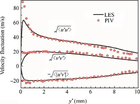
Fig.5 Squared Reynolds stress profile at x=260 mm.

Fig.6 Mean flow results.
Fig.6(a)shows the skin friction coefficient Cf,while Fig.6(b)is the wall pressure pwdistribution(normalized by incoming free-stream static pressure).The results are compared with the LES results of Touber and Sandham55,and reasonable agreements are achieved.The wavy profile of the skin friction may be due to the lack of statistical samples.We can see from the figure that the flow separates at x=295.32 mm and reattaches at x=334.67 mm,resulting a mean separation bubble length of about 39.4 mm.
Figs.7 and 8 show the comparison of the mean streamwiseˉU*and the wall-normal velocity profilesˉV*of LES predications and PIV measurements at five successive streamwise locations.Some noticeable influences of adverse pressure gradient on the development of the boundary layer's shape can be seen across the entire interaction zone.Overall,the LES results are in good agreements with the PIV data.The boundary layer thickening process is well captured according to the mean streamwise profile evolution.The wall-normal velocity also agrees well with the measured data,although the agreement is not as good as that of the streamwise velocity profiles since the PIV data could be less converged for the wall-normal velocity.Generally,the LES predictions and PIV measurements agree extremely well in both upstream and downstream of the interaction,while some discrepancies are observed in the interaction zone where the flow is unsteady and complex,thus difficult to simulate or measure accurately.
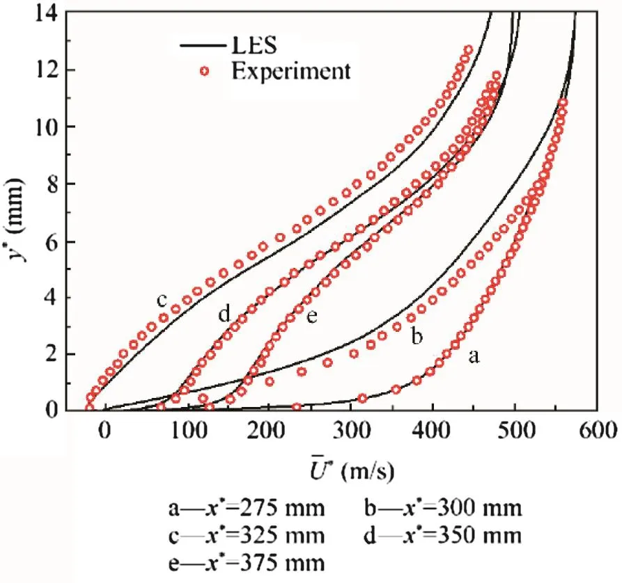
Fig.7 Mean streamwise velocity profiles at different streamwise locations.

Fig.8 Mean wall-normal velocity profiles at different streamwise locations.

Fig.9 Streamwise-velocity fluctuations profiles at different streamwise locations.

Fig.10 Wall-normal-velocity fluctuations profiles at different streamwise locations.

Fig.11 Reynolds shear-stress field profiles at different streamwise locations.

As for the instantaneous flow structure,Fig.12 shows the instantaneous numerical Schlieren(by using density gradient magnitude|?ρ|)and the streamwise velocity fluctuation at the plane of y+=15.The shock-wave system is clearly captured and the typical low-speed streaks of the equilibrium turbulent boundary layer can be clearly observed before entering the interaction region.The streaks are broken in the interaction region and gradually recovered after the reattachment.

Fig.12 Instantaneous flow structure,numerical Schlieren of shock-wave and boundary layer streaks.
In general,the LES results,including both the mean profile and the second-order turbulence statistics,agree well with the PIV measurements.Thus the ability of present LES to reproduce the complex flow field of SWTBLI is verified.On the other hand,as the PIV data are obtained from the median plane of the wind tunnel,this agreement also testifies that the experiment is close to being statistically two-dimensional and the wind tunnel corner flow has little impact in this case.
4.SparkJet control
Based on the validation of numerical method and CFD code in the above section,the LES is further used to study the SWTBLI flow with the SparkJet control as shown above.The SparkJet device is placed before the separation zone.The geometrical parameters of the configuration are chosen in reference to the real device in experiment.30For the purpose of the proof of concept,rectangular subdomain is adopted in present computations rather than the cylinder shape used in experiments due to the limitation of our grid patched structured code.By the physical intuition,the cavity volume should have a major influence on the actuator characteristics against the shape as the cavity volume directly influences the dynamical change of the pressure inside the cavity.However,the influence of the cavity shape remains for the further study.The energy deposition process of electrical discharge heating performed during the test is modeled by introducing an additional heating source in the total energy equation.
We adopted a relatively narrower span wise computational domain here to avoid redundant calculations and massive storage space of long time integration,and the non-control base flow with the same span wise length is also carried out for comparisons(not shown).The span wise length here is larger than the narrowest case presented in the LES of Touber and Sandham,58in which the results has been verified in details.The computation domain of the base flow is(Lx,Ly,Lz)=(256 mm,51 mm,14.0 mm),and the streamwise domain range is also[148,404]mm,which are the same as those in the above section.The center of the device is placed at x=280 mm,which is 1.5 nominal boundary layer thickness before the separation line.The throat size is(Lx,Ly,Lz)=(2 mm,1 mm,2 mm),while the cavity is a cube of length(Lx,Ly,Lz)=(6 mm,6 mm,6 mm).Fig.13 shows the geometry of the SparkJet actuator model in the present simulation.This control device geometry is comparable with that used in UIUC's experiment.30In the UIUC's experiment,the cavity volume is 183 mm3and jet is exhausted through a 0.83 mm diameter orifice,while in the present simulation the cavity volume is 216 mm3and the jet flow is exhausted through a squared throat of 4 mm.2The numbers of computational grids in each block are given in Table 4.

Fig.13 SparkJet control device geometry in present simulation.

Table 4 Total grid numbers of three computational domains.
The heating source pulse is distributed spherically from the center of the cavity domain and explicitly given by the following formula,

This model was proposed by Zheltovodov et al.59,60as the energy deposition(ED)model in their simulation.
In the formula above,the parameter q0decides the spark heating intensity,(x0,y0,z0)are the coordinates of the center of the heating source,(Rx,Ry,Rz)represent the energy concentration radiuses,f is the pulse frequency,and τ is the heating duration in each pulse.In the present simulation,the heating source is positioned at the center of the cavity cubic,the radiuses(Rx,Ry,Rz)are set as 2 mm,and non-dimensional heating intensity q0is 0.15.Integrating the heating source over time and space,we get the total added energy Q.The total deposited energy Q here is 8.9 J in a time duration of τ=20 μs.The choosing of the energy source parameters is also in reference to the UIUC's experiment.In the experiment,they tested three different energy levels E,e.g.,41 mJ,330 mJ,and 4.0 J,and the heating duration is also 20 μs.The simulation condition is comparable to the highest energy level case of the experiment.As we focused on the characteristics of a single-pulse,the pulse frequencyfis not involved here,and the flow field is sampled every 4 μs in a time span of 1000 μs after energy deposition starts.

Fig.14 Instantaneous numerical Schlieren of the controlled flow field and an enlarged view near the control device.
Fig.14 gives the instantaneous numerical Schlieren of the controlled flow field at the span wise middle plane and an enlarged view near the control device.The streamline in the cavity and near the throat is also shown,from which the interaction between the ejected jet flow and the main flow can be observed.Small shock lets can be seen ahead and near the jet flow.Also we can see that in the cavity,the air explodes from the center to the surrounding walls after the energy deposition process started.At the upper exit plane of the cavity domain,a jet stream is formed and ejected into the main flow.It can be seen that because of the high momentum of supersonic boundary layer,the jet is con fined in the near-wall region of the boundary layer.The height of the jet is about 10–20%of the local boundary layer thickness.However,it still has an obvious influence on the downstream interaction zone.Fig.15 gives the time history of the streamwise velocity variations U/Ueof three monitor points marked as'A,B,C'in the cavity domain(see Fig.14),which reveals the compression wave propagating from the center to the wall,and the oscillation may be caused by the interaction between the traveling wave and the reflected wave inside the cavity.

Fig.15 Time history velocity at three monitor points A,B and C in the cavity.

Fig.16 Maximum jet velocity and Mach number at the exit of the throat.
Fig.16 plots the maximum jet velocity and Mach number at the exit of the throat region.It can be seen that in a short time period after the energy deposition,the air in the cavity will expand and be ejected into the main flow at rapidly increased velocity up to the maximum peak value.Then the discharge velocity will gradually decline to the minimum value close to zero,which will be followed by a slow recovery phase.The highest jet velocity predicted from LES is about 446 m/s.The measurement of UIUC's experiment on SparkJet in a quiescent environment is also presented in Fig.16.As the control parameters in the present simulation are close to the highest energy level(4.0 J)case,and a corresponding peak jet speed is close to that of experimental data.However,the time history of maximum velocity from the LES prediction exhibits a more rapid decay rate than that of the experiments,which may be due to a larger jet exit area used in the present simulation.
Fig.17 shows the turbulence coherent structures identified by Q-criterion in the vicinity of the jet exit.In the incoming boundary layer in the upstream of the control device,the typical streamwise vortex patterns are identified.Then the main flow interacts with the jet from the cavity and complex vortex structures are generated.Fig.18 shows the enlarged view near the exit,where a rectangular vortex ring(resulting from the jet in cross- flow interactions)can be clearly seen.The three dimensional streamlines near the throat plotted as the yellow ribbon reveal the nature of mixing flow in this region.Around the jet,a horseshoe vortex can be identified,which is similar to the structure in blunt body round flow.

Fig.17 Turbulence coherent structures in the boundary layer.

Fig.18 Turbulence coherent structures and streamlines near jet exit.
Fig.19 gives the slices at different streamwise locations across the control device,which are contoured by density with the projected streamlines shown.In these figures,the evolution of a pair of counter-rotating streamwise vortexes in the boundary layer is clearly observed.The structures are very similar to the wake of vortex generator.32,61Fig.20 shows the time averaged streamwise velocity profiles of mid-span plane at different streamwise locations across the control device correspondingly,and the velocity profiles are obviously fuller than that of the uncontrolled case,which indicates that the mixing process enhances the boundary layer's ability to resist flow separation.The flow topology around the exit and in the wake shows that the SparkJet plays as a virtual vortex-generator and promotes flow mixing inside the boundary layer,thus enhancing its ability to resist flow separation.
Fig.21 shows the time and the spanwise-averaged skin friction coefficient variations along the streamwise direction.Compared with the uncontrolled base flow,the flow separation is delayed,resulting in an overall separation length reduction.The mean separation bubble length of the control case study is 31 mm,about 35%decrease against that of the uncontrolled case.

Fig.19 Slices at six different streamwise locations across throat.

Fig.20 Time averaged streamwise velocity profile evolution.

Fig.21 Time and span wise averaged skin friction coefficients variations along the streamwise direction.
5.Conclusions
(1)Large-eddy simulation of a Ma=2.3 shock-wave generated by 8°wedgeimpinging onto a spatially developing turbulent boundary layer along a flat plate is carried out.The numerical approaches and the simulation results are systematically validated with experimental measurements in the same flow condition,which establishes the database of the basic SWTBLI flow field.
(2)Based on this,the''SparkJetquot;control technique developed for the SWTBLI flow is further studied using LES.The configuration of the control device is modeled in reference to the experiments with similar configuration parameters.The single-pulse characteristics of the control mechanism are analyzed and the effects of the SparkJet on the main SWTBLI flow are visualized.
(3)The maximum jet velocity time history agrees qualitatively well with the experiments and a maximum jet velocity of 446 m/s is predicted,which is close to that of experimental measurement.By exerting the control device,the flow separation is delayed noticeably and the average length of the separation bubble also reduces by about 35%,and this proves the effectiveness of the SparkJet control technique on suppressing the flow separation occurred in SWTBLI flows.
Acknowledgements
This work was supported by the National Natural Science Foundation of China (Nos. 11302012, 51420105008,51476004,11572025 and 51136003)and the National Basic Research Program of China(No.2012CB720205).The computational time for the present study was provided by the UK Turbulence Consortium(EPSRC grant EP/L000261/1)and the simulations were run on the UK High Performance Computing Service ARCHER.We also would like to acknowledge the University of the West of England for hosting the first author to carry out the initial simulation work.
1.Dolling DS.Fifty years of shock-wave/boundary-layer interaction research:what next.AIAA J 2001;39(8):1517–31.
2.Ferri A.Experimental results with aerofoil tested in high speed tunnel at Guidonia.Washington,D.C.:NASA;1940,Report No.:NACA TM 946.
3.Settles GS,Dodson LJ.Hypersonic shock/boundary-layer interaction database.Washington,D.C.:NASA;1991,Report No.:NASA STI/Recon Technical Report 93:24526.
4.Delery JM,Panaras AG.Shock wave boundary-layer interaction in high Mach number flows.Paris:Advisory Group for Aerospace Research and Development;1996,Report No.:AGARD Advisory Report AR-319.
5.Ma L,Lu LP,Fang J,Wang QH.A study on turbulence transportation and modification of Spalart-Allmaras model for shock-wave/turbulent boundary layer interaction flow.Chin J Aeronaut 2014;27(2):200–9.
6.Green JE.Interactions between shock waves and turbulent boundary layers.Prog Aerosp Sci 1970;11:235–340.
7.Adamson Jr TC,Messiter AF.Analysis of two-dimensional interactions between shock waves and boundary layers.Annu Rev Fluid Mech 1980;12(1):103–38.
8.Delery JM.Shock phenomena in high speed aerodynamics:still a source of major concern.Aeronaut J 1999;103(1019):19–34.
9.Knight DD,Yan H,Panaras AG,Zheltovodov AA.Advances in CFD prediction of shock wave turbulent boundary layer interactions.Prog Aerosp Sci 2003;39(2):121–84.
10.Babinsky H,Harvey JK.Shock wave-boundary-layer interactions.Cambridge:Cambridge University Press;2011.
11.Babinsky H,Ogawa H.SBLI control for wings and inlets.Shock Waves 2008;18(2):89–96.
12.Titchener N,Babinsky H.Shock wave/boundary-layer interaction control using a combination of vortex generators and bleed.AIAA J 2013;51(5):1221–33.
13.Georgiadis NJ,Rizzetta DP,Fureby C.Large-eddy simulation:current capabilities,recommended practices,and future research.AIAA J 2010;48(8):1772–84.
14.Moin P,Mahesh K.Direct numerical simulation:a tool in turbulence research.Annu Rev Fluid Mech 1998;30(1):539–78.
15.Garnier E,Adams NA,Sagaut P.Large eddy simulation for compressible flows.Berlin:Springer Scienceamp;Business Media;2009.p.1–10.
16.Garnier E,Sagaut P,Deville M.Large eddy simulation of shock/boundary-layer interaction.AIAA J 2002;40(10):1935–44.
17.Loginov MS,Adams NA,Zheltovodov AA.Large-eddy simulation of shock-wave/turbulent-boundary-layer interaction.J Fluid Mech 2006;565:135–69.
18.Teramoto S.Large-eddy simulation of transitional boundary layer with impinging shock wave.AIAA J 2005;43(11):2354–63.
19.Clemens NT,Venkateswaran N.Low-frequency unsteadiness of shock wave/turbulent boundary layer interactions.Annu Rev Fluid Mech 2014;46:469–92.
20.Viswanath PR.Shock-wave-turbulent-boundary-layer interaction and its control:a survey of recent developments.Sadhana 1988;12(1–2):45–104.
21.Lin JC.Review of research on low-profile vortex generators to control boundary-layer separation.Prog Aerosp Sci 2002;38(4):389–420.
22.Lu FK,Li Q,Liu CQ.Microvortex generators in high-speed flow.Prog Aerosp Sci 2012;53:30–45.
23.Blinde PL,Humble RA,van Oudheusden BW,Scarano F.Effects of micro-ramps on a shock wave/turbulent boundary layer interaction.Shock Waves 2009;19(6):507–20.
24.Gefroh D,Loth E,Dutton C,Hafenrichter E.Aeroelastically deflecting flaps for shock/boundary-layer interaction control.J Fluids Struct 2003;17(7):1001–16.
25.Srinivasan KR,Loth E,Dutton CJ.Aerodynamics of recirculating flow control devices for normal shock/boundary-layer interactions.AIAA J 2006;44(4):751–63.
26.Popkin SH,Taylor TM,Cybyk BZ.Development and application of the SparkJet actuator for high-speed flow control.Johns Hopkins APL Technical Digest 2013;32(1):404–18.
27.Doerffer PP,Bohning R.Shock wave-boundary layer interaction control by wall ventilation.Aerosp Sci Technol 2003;7(3):171–9.
28.Pasquariello V,Grilli M,Hickel S,Adams NA.Large-eddy simulation of passiveshock-wave/boundary-layerinteraction control.Int J Heat Fluid Flow 2014;49:116–27.
29.Land HB,Grossman KR,Cybyk BZ,VanWie DM.Solid sate supersonic flow actuator and method of use.United States Patent US7988103;2011 Aug 2.
30.Reedy TM,Kale NV,Dutton CJ,Elliot GS.Experimental characterization of apulsed plasmajet.AIAA J2013;51(8):2027–31.
31.Belinger A,Naude′N,Cambronne JP,Caruana D.Plasma synthetic jet actuator:electrical and optical analysis of the discharge.J Phys D Appl Phys 2014;47(34):345202.
32.Caruana D,Barricau P,Gleyzes C.Separation control with plasma synthetic jet actuators.Int J Aerodyn 2013;3(1):71–83.
33.Cybyk BZ,Grossman KR,Wilkerson J,Chen J,Katz J.Singlepulse performance of the sparkjet flow control actuator.Reston:AIAA;2005,Report No.:AIAA-2005-0401.
34.Cybyk BZ,Simon DH,Land H,Chen J,Katz J.Experimental characterization of a supersonic flow control actuator.Reston:AIAA;2006,Report No.:AIAA-2006-0478.
35.Cybyk BZ,Wilkerson JT,Grossman KR.Performance characteristics of the sparkjet flow control actuator.Reston:AIAA;2004,Report No.:AIAA-2004-2131.
36.Jin D,Li YH,Jia M,Song HM,Cui W,Sun Q,et al.Experimental characterization of the plasma synthetic jet actuator.Plasma Sci Technol 2013;15(10):1034–40.
37.Grossman KR,Cybyk BZ,van Wie DM.Sparkjet actuators for flow control.Reston:AIAA;2003,Report No.:AIAA-2003-0057.
38.Haack SJ,Taylor TM,Cybyk BZ,Foster C,Alvi F.Experimental estimation of SparkJet efficiency.Reston:AIAA;2011,Report No.:AIAA-2011-3997.
39.Haack SJ,Land HB,Cybyk BZ,Ko HS,Katz J.Characterization of a high-speed flow control actuator using digital speckle tomography and PIV.Reston:AIAA;2008,Report No.:AIAA-2008-3759.
40.Ko HS,Haack SJ,Land HB,Cybyk BZ,Katz J,Kim HJ.Analysis of flow distribution from high-speed flow actuator using particle image velocimetry and digital speckle tomography.Flow Meas Instrum 2010;21(4):443–53.
41.Reedy TM,Kale NV,Dutton JC,Elliott GS.Experimental characterization ofapulsed plasmajet.AIAA J2013;51(8):2027–31.
42.Narayanaswamy V,Raja LL,Clemens NT.Control of a shock/boundary-layer interaction by using a pulsed-plasma jet actuator.AIAA J 2012;50(1):246–9.
43.Narayanaswamy V,Shin J,Clemens NT,Raja LL.Investigation of plasma-generated jets for supersonic flow control.Reston:AIAA;2008,Report No.:AIAA-2008-0285.
44.Vreman B.Direct and large-eddy simulation of the compressible turbulent mixing layer dissertation.Enschede:University of Twente;1995.
45.Inagaki M,Tsuguo K,Yasutaka N.A mixed-time-scale SGS model with fixed model-parameters for practical LES.J Fluids Eng 2005;127(1):1–13.
46.Li Q.Numerical study of Mach number effects in compressible wall-bounded turbulence dissertation.Southampton:University of Southampton;2003.
47.Carpenter MH,Nordstro¨m J,Gottlieb D.A stable and conservative interface treatment of arbitrary spatial accuracy.J Comput Phys 1999;148(2):341–65.
48.Gottlieb S,Shu CW.Total variation diminishing Runge-Kutta schemes.Math Comput Am Math Soc 1998;67(221):73–85.
49.Yee HC,Sandham ND,Djomehri MJ.Low-dissipative high-order shock-capturing methods using characteristic-based filters.J Comput Phys 1999;150(1):199–238.
50.Sandham ND,Li Q,Yee HC.Entropy splitting for high-order numerical simulation of compressible turbulence.J Comput Phys 2002;178(2):307–22.
51.Ducros F,Ferrand V,Nicoud F,Weber C,Darracq D,Gacherieu C,et al.Large-eddy simulation of the shock/turbulence interaction.J Comput Phys 1999;152(2):517–49.
52.Yao YF,Shang Z,Castagna J,Sandham ND,Johnstone R,Sandberg RD,et al.Re-engineering a DNS code for highperformance computation of turbulent flows.Reston:AIAA;2009,Report No.:AIAA-2009-0566.
53.Poinsot TJ,Lelef SK.Boundary conditions for direct simulations of compressible viscous flows.J Comput Phys 1992;101(1):104–29.
54.Fang J,Yao YF,Zheltovodov AA,Li ZR,Lu LP.Direct numerical simulation of supersonic turbulent flows around a tandem expansion–compression corner.Phys Fluids 2015;27(12),125104-1-27.
55.Touber E,Sandham ND.Large-eddy simulation of low-frequency unsteadiness in a turbulent shock-induced separation bubble.Theor Comput Fluid Dyn 2009;23(2):79–107.
56.Touber E,Sandham ND.Large-eddy simulations of an oblique shock impinging on a turbulent boundary layer:low-frequency mechanisms18th international shock interaction symposium,2008.2008.
57.Dupont P,Haddad C,Debieve JF.Space and time organization in ashock-induced separated boundarylayer.JFluidMech 2006;559:255–77.
58.Touber E,Sandham ND.Low-order stochastic modelling of lowfrequency motions in reflected shock-wave/boundary-layer interactions.J Fluid Mech 2011;671:417–65.
59.Adelgren RG,Elliott GS,Knight DD,Zheltovodov AA,Beutner TJ.Energy deposition in supersonic flows.Reston:AIAA;2001,Report No.:AIAA-2001-0885.
60.Zheltovodov AA,Pimonov EA,Knight DD.Numerical modeling of vortex/shock wave interaction and its transformation by localized energy deposition.Shock Waves 2007;17(4):273–90.
61.Caruana D,Barricau P,Hardy P,Cambronne JP,Belinger A.The,''plasma synthetic jetquot;actuator.Reston:AIAA;2009,Report No.:AIAA-2009-1307.
Yang Guangis a Ph.D.student at School of Power and Energy,Beihang University.He received his B.S.degree from Beihang University in 2011.His area of research includes shock-wave/boundary layer interaction,flow control,and large-eddy simulation.
Yao Yufengis a professor in aerospace engineering and head of Engineering Modelling and Simulation Research Group at the University of the West of England,Bristol,United Kingdom.He has vast research interests including turbulent flow and heat transfer using advanced and high-fidelity numerical methods.
Fang Jianis currently a lecturer at School of Energy and Power Engineering,Beihang University.His research interests are high-order CFD method,high-speed gas dynamics and complex turbulence mechanism and modeling.
25 May 2015;revised 12 August 2015;accepted 25 December 2015
Available online 10 May 2016
Large-eddy simulation;
Shock-wave;
Turbulent boundary layer;
Interaction;
SparkJet control
?2016 Chinese Society of Aeronautics and Astronautics.Production and hosting by Elsevier Ltd.This is an open access article under the CCBY-NC-ND license(http://creativecommons.org/licenses/by-nc-nd/4.0/).
*Corresponding author.Tel.:+86 10 82316455.
E-mail addresses:g.y_1990@163.com(G.Yang),Yufeng.Yao@uwe.ac.uk(Y.Yao),fangjian@buaa.edu.cn(J.Fang).Peer review under responsibility of Editorial Committee of CJA.
 CHINESE JOURNAL OF AERONAUTICS2016年3期
- CHINESE JOURNAL OF AERONAUTICS的其它文章
- Optimization on cooperative feed strategy for radial–axial ring rolling process of Inco718 alloy by RSM and FEM
- Measuring reliability under epistemic uncertainty:Review on non-probabilistic reliability metrics
- Optimum blade loading for a powered rotor in descent
- Experimental study of ice accretion effects on aerodynamic performance of an NACA 23012 airfoil
- Parachute dynamics and perturbation analysis of precision airdrop system
- Simulative technology for auxiliary fuel tank separation in a wind tunnel