Remaining useful life estimation for deteriorating systems with time-varying operational conditions and condition-specific failure zones

Li Qi,Gao Zhanbao,Tang Diyin,Li Baoan

School of Automation Science and Electrical Engineering,Beihang University,Beijing 100083,China

Remaining useful life estimation for deteriorating systems with time-varying operational conditions and condition-specific failure zones

Li Qi,Gao Zhanbao,Tang Diyin*,Li Baoan

School of Automation Science and Electrical Engineering,Beihang University,Beijing 100083,China

Dynamic time-varying operational conditions pose great challenge to the estimation of system remaining useful life(RUL)for the deteriorating systems.This paper presents a method based on probabilistic and stochastic approaches to estimate system RUL for periodically monitored degradation processes with dynamic time-varying operational conditions and conditionspecific failure zones.The method assumes that the degradation rate is influenced by specific operational condition and moreover,the transition between different operational conditions plays the most important role in affecting the degradation process.These operational conditions are assumed to evolve as a discrete-time Markov chain(DTMC).The failure thresholds are also determined by specific operational conditions and described as different failure zones.The 2008 PHM Conference Challenge Data is utilized to illustrate our method,which contains mass sensory signals related to the degradation process of a commercial turbofan engine.The RUL estimation method using the sensor measurements of a single sensor was first developed,and then multiple vital sensors were selected through a particular optimization procedure in order to increase the prediction accuracy.The effectiveness and advantages of the proposed method are presented in a comparison with existing methods for the same dataset.

1.Introduction

The discipline of prognostic and health management(PHM)brings about the idea of using monitoring techniques and data analysis methods to assess the reliability of a system in its life cycle and to determine the occurrence of failure.Estimating the remaining useful life(RUL)is considered as the core and always a major challenge in PHM.Once accurate prognostic results are available,appropriate health management actions such as maintenance and logistical support are able to perform in time.For aircraft or aerospace vehicles,accurate RUL estimation not only means much to the cost savings,but more importantly,it is of great significance in ensuring system reliability and preventing disaster.The current techniques for RUL estimation can be roughly classified into physical-based approaches,data-driven approaches and their combinations.For complex systems such as nuclear power systems,aircraft engines,flight control systems,etc.,it is too complicated to map their precise physics to their exact failure mechanisms,thus data-driven approaches are good alternatives to accomplish the prognostic tasks.

Many data-driven approaches for RUL estimation employ data fitting methods including machine learning and statistical based methods to model the system deterioration process.When developing an appropriate degradation model to predict the system's future behavior,the uncertainty underlying the deterioration process is an important issue that should be taken into serious account.The existing methods have broadly presented two ways to describe the uncertainty in a degradation model.One is using probabilistic methods,in which the deterioration phenomenon is considered to have certain random behavior which is often characterized by probability laws,e.g.,normal distribution1–4,or by stochastic models,e.g.,Wiener processes5–7,Gamma processes8,9,inverse Gaussian processes10,11,etc.The other can be referred to as parameter updating strategies,which updates the models parameter by newly available data acquired from currently functioning individuals.Gebraeel et al.6developed a Bayesian method to update the stochastic parameters of exponential degradation models using real-time condition monitoring information.Variations of this work have been investigated in many literatures,e.g.,Elwany12,Bian13,You14and Si et al.15Following the Bayesian-based updating principals,Ye and Chen10developed an updating procedure for inverse Gaussian processes;Si et al.7proposed a Bayesian recursive filter to update the drift coefficient in the Wiener process,and further,this recursive filter was improved in the study of Si et al.16to deal with a general nonlinear degradation model.Besides Bayesian-based updating approaches,many other updating approaches have also been reported,e.g.,Chen et al.17utilized both the current observations and the future prediction results obtained by support vector machine to update the system model parameters.

Various reasons may contribute to the uncertainties in a deterioration process;however,with all kinds of reasons,the influence of time-varying operational conditions(or environmental conditions)has not received enough attention.As noted by Bian et al.,18most degradation models assume that the operational conditions are invariant,or without affecting the deterioration process.However,this is not always true in real engineering applications.The operational conditions usually vary with environmental changes or operating mode conversions,and in most cases,they exerted non-trivial effects on the process of deterioration.Examples can be found in inertial navigation systems19,flight control systems20,smart power grids21and other smart structures.

In recent years,a few probabilistic methods considering the effect of operational conditions on degradation processes have been proposed.Liao and Tian22developed a Bayesian updating technique for Wiener process-based degradation models to accommodate piecewise constant operating conditions.Bian and Gebraeel23proposed a tangent approximation method to estimate RUL for a Wiener process-based degradation model under a continuous deterministic environmental profile.To deal with dynamic environmental conditions,Kharoufeh and Cox24considered a random environment characterized by a continuous-time Markov chain,and Kharoufeh et al.25further extended this method to semi-Markov-based random environment.Si et al.26predicted residual storage life for systems with switches between the working state and the storage state,considering a continuous-time Markov chain to describe the state sojourns and switches.In above methods,the quantified effect of operational conditions on degradation processes only comes from specific operational conditions,but the effect resulted from the transition between different operational conditions has not been included.Among limited contributions which combine both effects,Bian et al.18studied a complex situation in which the failure rates are determined by environmental conditions,and the degradation signal exhibits upward or downward jumps at environment transition epochs.In their model,the jump magnitudes are supposed to be deterministic quantities and the degradation rates are the main factor in deterioration.However,in some situations,the jump magnitude is more of a random variable than a deterministic quantity,and it leads the deterioration trend especially when the operational condition changes frequently.

In this paper,we will focus on estimating RUL using probabilistic methods for degrading systems under time-varying operational conditions and subject to equidistant condition monitoring.The dynamics of the time-varying operational conditions will be considered and described by a discretetime Markov chain(DTMC).The influence from both the operational conditions and the transitions of operational conditions on degradation processes will be quantified and incorporated in the degradation model.In order to validate our RUL estimation method,we use 2008 PHM Conference Challenge Data27,a mass run-to-fail dataset simulated from a model of a realistic large commercial turbofan engine,to present our algorithm,to analyze the results,as well as to compare the proposed method with other existing approaches for the same dataset.We select several benchmark methods dealing with this data for comparison purposes:similarity-based regression approach by Wang et al.,28neural networks approach by Heimes29and Peel30,and Wiener process-based approach by Son et al.31Our method is different from all existing methods dealing with this dataset in at least three aspects.Firstly,instead of using fusion methods to eliminate different influences resulted from different operational conditions,we quantify these differences according to different operational conditions and different transitions of operational conditions.Secondly,we consider condition-specific failure zones instead of a general failure threshold.To our knowledge,we are the first to consider different failure mechanisms according to different operational conditions.Not only does our illustrative example present such pattern,but also this consideration is more realistic and appropriate in many real applications.For example,a degraded system may not be capable of operating under harsh conditions,but it may operate safely under mild conditions.Thirdly,although sensor measurements from various sensors are available,our proposed method enables RUL estimation using each single sensor,which allows us to develop an optimization procedure to select the sensors that contribute most to the accuracy of prognostics.

The remainder of the paper is organized as follows.In Section 2,the 2008 PHM Conference Challenge Data is introduced.Methods for preliminary sensor selection and failure zone construction are presented in Section 3.In Section 4,the model to describe the degradation process under dynamic operational conditions is developed.RUL estimation methods and corresponding estimation results,as well as the optimization procedure to select the most contributive sensors are discussed in Section 5.Conclusions and future works are given in Section 6.

2.Motivating problem

In this paper,we will illustrate our RUL estimation method using the 2008 PHM Conference Challenge Data.This dataset describes the run-to-failure process of a realistic large commercial turbofan engine by documenting the time series data of its multiple sensors,which is generated via a simulation tool based on athermo-dynamical model.27Though many researchers28–31proposed distinguished RUL estimation methods for this dataset,they conducted their research on the basis of eliminating the differences of operational conditions;however,in our method,we will quantify those differences in the excavation of degradation features,the construction of failure thresholds,and the development of the degradation model.The performance of our method is compared with that of those benchmark methods to show its advantages and potential.

2.1.Data layout

The dataset consists of multivariate sensor data collected at the end of each equidistant cycle.It is further divided into the training dataset and the testing dataset,each containing 218 units.Each unit starts with different degrees of initial wear and manufacturing variation which is unknown to the user.The sensor data for each cycle of each unit includes the unit ID,the time cycle,3 values for the operational settings and 21 values for 21 sensor measurements.The sensor measurements are contaminated with noise.As shown in Table 1,three operational settings affect engine degradation behavior,which results in six different operational conditions(OC).Fig.1 shows an example(Unit 1 in the training dataset)of the sensor measurements and the dynamic process of corresponding operational conditions.It shows that the operational conditions change quite randomly during the degradation process,and with this random process,it is hard to discover the degradation trend directly from the time series sensor measurements.

The training dataset is used for developing RUL estimation methods,in which the degradation process runs until the system fails.In the testing dataset,the sensor measurement endsat some time prior to system failure,and then the units with partial degradation information are used to test and validate the developed RUL estimation methods.We will predict the number of remaining operating cycles before system fails for the testing dataset and compare our results with those of the existing methods.

Table 1 Six different operational conditions(OC).

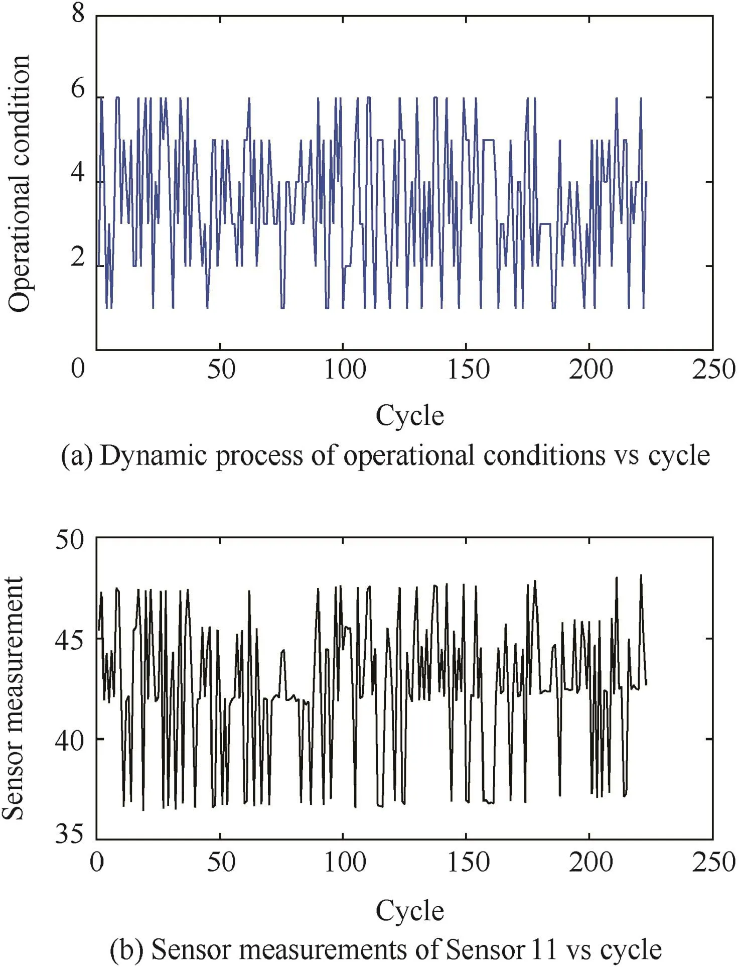
Fig.1 Sensor measurements of Sensor 11 and corresponding operational conditions for training Unit 1.

2.2.Performance evaluation method

Performance metrics are functions of prediction errors.Traditional performance metrics32concentrate on prediction accuracy which can meet the basic requirement of performance evaluation.However,these metrics may not be enough to meet the special needs of prognostics.Therefore,in this paper,some basic traditional performance metrics as well as a specific performance evaluation system proposed by Saxena et al.33will be utilized to evaluate our method and for comparison purposes.The prediction error is noted asRULl(l=1,2,...,L),wherelis the total number of predictions,andand RULlare the predicted and the true RUL for Unit l,respectively.

Traditional performance metrics evaluate how close the prediction is to the truth,such as bias,root squared error(RSE),and mean squared error(MSE),which are given by

Since prediction error can be negative or positive,Bias may mislead the accuracy judgment.Therefore,RSE and MSE are chosen as the performance metrics for our algorithm as they rely on the absolute value of prediction errors.The two metrics are used as the performance metrics in Refs.29,30,which facilitate performance comparison as well.

To finish prognostic task in PHM,since the key aspect is to avoid failure,early prediction is generally more desirable than late prediction.Traditional performance metrics are universal for prediction problems,but when two prediction algorithms have similar accuracy,the traditional metrics are incapable of distinguishing the better one which predicts failure earlier.On the other hand,too early predictions may on the contrary introduce too much economic burden.Hence,Saxena et al.33proposed a scoring algorithm to address this specific requirement.It is an asymmetric function stressing heavier penalties on late prediction than early prediction and the penalty grows exponentially with increasing error.The evaluation metric is expressed as

The asymmetric preference is decided by parameter{φ1,φ2}in the function.In order to capture the preference for early results well and tune a reasonable extent of such preference,the recommended setting of the parameter is φ1=10,φ2=13.The setting is also used in Refs.28,31which will be compared to our prognostic algorithm in the following section.

The asymmetric score metric has the ability of distinguishing early predictions from late predictions,but it is sensitive to abnormal samples which may influence the whole evaluation.Therefore,we choose both traditional performance metrics and asymmetric score metric to evaluate our prediction results,in order to provide a more valuable and general assessment of prediction performance.

3.Preliminary sensor data analysis

After obtaining the raw sensor data,it is of first importance to excavate data features related to the degradation,and then identify the health indicator(degradation indicator)and the failure mechanism in order to establish the mapping between the degradation and the system failure.

The health indicators can be broadly classified into two kinds:the physical health indicator and the virtual health indicator.The physical health indicator directly comes from physical signals and it has physical interpretations,while the virtual health indicator usually comes from synthetic approaches which transform the multi-dimensional sensory signals into lower dimensional indicators.In real applications,physical health indicators used in prognostic practices can be shown in many forms,such as battery impedance34,magnitude of vibration signal,etc.,5while virtual health indicators are constructed by approaches such as regression,28principal component analysis,etc.31According to our knowledge,for the 2008 PHM Conference Challenge Data,all existing methods resorted to virtual health indicators.However,in this paper,we will excavate physical health indicators directly from the sensor data.

3.1.Feature analysis of sensor data

Before we establish health indicators for the degradation process,we should first select the sensors whose signals contain degradation information.The Challenge Data provides 21 sensor measurements at each cycle for each unit.For any specific operational condition,the plots of the sensor measurements collected under such operational condition for each of the 21 sensors are gathered in the time order to show the trend of the system's deterioration.Take OC 3 as an example,we plot in Fig.2 the sensor measurements collected at OC 3 for all 218 training units.From those distinguishing features shown in Fig.2,we split all sensors into 4 categories(see Table 2 for detailed description).

It is clear that the sensors in the Constant type and Anomaly type do not show apparent degenerated feature as time proceeds,thus they are not suitable for degradation modeling.Except these sensors,all the rest exhibit some degradation trend over cycles.Sensors in the Trended category exhibit an upward or downward trend when the system operated to the end of its life.More importantly,for the same sensor,similar trends with the same progressing direction(upward or downward)are shown in all units.For example,as shown in Fig.3(a),the degradation revealed by the sensor measurements of Sensor 11 under OC 3 for training Units 1–3 shows the same upward trend.This consistent trend among all individuals gives us an opportunity to build physical health indicators based on sensor measurements of a single sensor and determine failure zones for the prediction of failure.However,on the other hand,we find that sensors in the Divergent category do not present such consistent trend among all individuals.For instance,as Fig.3(b)shows,sensor measurements of Sensor 9 for Unit 1 show an upward trend,while the trend for Unit 2 is downward,and for Unit 3 it is more of in a stable pattern.Their differences increase over time especially at the end of life.This inconsistency makes it almost impossible in our method to find appropriate failure zones based on sensor measurements.Although excluding sensors with divergent trend for RUL prediction will cause potential loss of degradation information,inappropriate determination of failure mechanism may also reduce model sensitivity and lead to poor prediction.Therefore,only eight trended sensors are selected as the candidate sensors in our method.However,the solution to utilize sensors with divergent trend deserves more future works of our research.

The selected sensor measurements are the physical health indicators in the degradation model development.Though those sensor measurements may contain noise,since the failure zones will be constructed based on these sensor measurements,we will use the terms''sensor measurementquot;and''degradation statequot;interchangeably in the remainder of this paper.

3.2.Failure zone construction

Fig.2 Time series sensor measurements of 21 sensors under OC 3 for all 218 training units.

Table 2 Four different categories for 21 sensors based on features of sensor measurements.

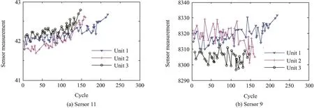
Fig.3 Time series sensor measurements of Sensors 11 and 9 for training Units 1–3 under OC 3.

Failure mechanism is the next issue we should address before RUL estimation.Many literatures use a deterministic failure threshold to identify failures.When the degradation state crosses this threshold,failure occurs.However,this is not always the case in real practices.Sometimes it is hard to find a specific value for the failure threshold.For this Challenge Data,we plot the sensor measurements of Sensor 11 at the failure time in Fig.4 according to different operational conditions.As the crosses show in each subfigure,the sensor measurements at the failure time seem to form a zone.Thus,we consider condition-specific failure zones instead of a general failure threshold for this problem.

Fig.4 Sensor measurements of Sensor 11 at initial and failure time for all training units.

Due to the fact that failure samples are scarce for some operational conditions,we also consider sensor measurements that are observed several cycles before the failure time when constructing failure zones.Here we define a failure state setfor each selected Sensorand each OC k(k=1,2,...,m),where m is the total number of different operational conditions.Let Yl,s(n)be the observed sensor measurement for selected Sensor s and Unit l(l=1,2,...,L)at the cycle time tn=nh(n=1,2,...)where h is the cycle length.We first collect the sensor measurements Yl,s(nl,s-a),Yl,s(nl,s-a+1),...,Yl,s(nl,s)for Sensor s,where tl,s=nl,sh is the failure time for Sensor s and Unit l,and a a predetermined integer.The specific failure state setis then formed by those collected sensor measurements found under OC k.

In this paper,without loss of generality,we de fine a=5.As an example,we plot the sensor measurements of Sensor 11 in setby solid circles in Fig.4.The triangles in Fig.4 are the initial sensor measurements found belonging to Sensor 11 for all training units.From Fig.4,we can also observe that the deterioration really happens and the sensor measurements perform well as health indicators.Fig.5 shows the normal probability plots for the sensor measurements in eachThe probability plots give a statistical proof that the sensor measurements in eachare normally distributed,following the law(k=1,2,...,6).Note that any other probability law can be considered,as long as the statistical evidence supports.

Fig.5 Probability plots for sensor measurements of Sensor 11 in each failure state set

Similar procedures are also applied to analyzingfor each candidate Sensor s inWe find that normal law applies to any failure state setTherefore,we determine the failure zone Ωs,kfor each selected Sensorand each OC k by the upper and lower boundaries:

The upper and lower boundaries of Sensor 11 are presented by lines in Fig.4.As shown in Fig.4,the failure zones Ωs,kare able to cover the majority of failure samples.The different failure standards we consider according to different operational conditions are realistic and appropriate,for example,deteriorated system may not be able to function under harsh operational conditions,but it may work safely under mild conditions.In the following RUL estimation method,we assume that the failure time of a unit is the first time when the sensor measurement enters the failure zone.However,we also notice that the first entering time is not always the actual failure time.In fact,some units may wander in the failure zone for a while before actually fail,some units may go out of the failure zone and then come back to fail,and some units may even fail before entering the failure zone.The prediction accuracy will surely be improved if the failure mechanism can be more precisely described,which can be a suitable topic for our future research.

4.Degradation modeling

In this section,we will present a degradation model to describe the time series degradation process for any selected sensor subject to condition monitoring at equidistant operating cycles.The degradation process is affected by time-varying operational conditions which vary stochastically according to a DTMC.

4.1.Modeling dynamic process of operational conditions

Let Z(n)be the operational condition at time tn=nh,which can be one and only one state of a set C={1,2,...,m},and for the challenge dataset,m=6.Under periodically monitored situation,we assume that the operational condition evolves stochastically according to a DTMC,with transition probabilities Prijgiven by

The one-step transition probabilities Prijfrom one operational condition to anther within one cycle can be estimated by

where Πijis the total number of transitions from OCito OC j in the whole training dataset,and Πithe total number of times that the system is found under the OC i.Note that we assume the cycle length h is small enough to ensure that only one transition could happen within one cycle.

We notice from above matrix that for this dataset the DTMC is an irreducible ergodic chain.Therefore,limiting probabilitiesexist and can be calculated by the following system of linear equations

The results of limiting probabilities for this dataset are listed in Table 3.The probabilities are almost the same with the actual frequencies for all operational conditions,demonstrating that DTMC is an appropriate stochastic model to describe the dynamic process of the operational conditions.

4.2.Modeling degradation process under time-varying operational conditions

We assume that the system degradation is determined by two processes.One is the gradual degradation under invariant operational conditions,and the other is the system state jumps caused by transitions of operational conditions.In our degradation model,the former process is described by a degradation rate us(Z(n))under specific operational condition Z(n)at time t,t∈(nh,(n+1)h],where s denotes Sensor s,and the latter process uses a function Js(Z(n-1),Z(n))to describe the magnitude of state jumps right after the transition from Z(n-1)to Z(n)within cycle interval((n-1)h,nh].We assume both us(Z(n))and Js(Z(n-1),Z(n))are random variables.In some existing literatures,in order to facilitate mathematical analysis,the degradation rate is supposed to be nonnegative.17,22,23We consider that degradation rates can be any value and the jumps can be either upward or downward in our degradation model.This assumption includes in the degradation model not only the actual deterioration leading the system to a more deteriorated state but also some self-recovering mechanisms which can be initiated by specific operational conditions or transitions of operational conditions.Such self-recovering mechanism can correspond,for example,to the minor maintenance activity such as lubrication within systems' working cycles,intense working load transferring to light working load,etc.

Table 3 Limiting probabilities and actual frequencies for six operational conditions.

We also assume that the transition of operational conditions is the main factor to influence the system degradation,which means,when the transition of operational conditions happens within an operating cycle,we only consider the state jumps.To valid this assumption,the cycle length h has to be small enough in order to ensure that only one transition could happen within one cycle and the accumulated deterioration caused by ordinary degradation rates is not capable of reaching a comparable magnitude to state jumps.This assumption greatly simplifies the degradation model and the RUL estimation method,and it is supported by this dataset.For example,in Fig.6,we plot the sensor measurements of Sensor 11 found under OC 3 for training Unit 139.The circles with dotted lines represent the change of degradation state under invariant OC 3 within adjacent cycles.From the whole run-to-failure process of training Unit 139,we can observe that degradation process under invariant OC 3 makes very limited contributions to the whole deterioration.

Based on above considerations,let Ys(n)be the observed sensor measurement of any selected Sensor s at time tn=nh,and let Ds(n)=Ys(n)-Ys(n-1)be the degradation increment within cycle interval((n-1)h,nh],then the degradation model for each selected sensor s can be described as

Compared with the existing degradation models,the proposed model is similar to the one presented by Bian et al.18but distinguishes itself in the following four aspects.Firstly,the magnitude of state jump Js(Z(n-1),Z(n))in our model is not a deterministic quantity but a random variable which can follow any arbitrary distributions.Secondly,the degradation rate us(Z(n))can be negative in order to embrace possible self-recovering mechanisms.Thirdly,we consider a periodically condition-monitored situation so that the continuous degradation process is discretized on the time axis.Last but the most important,we assume that the transition of operational conditions is the most prominent factor to influence the degradation process,which is appropriate for many real applications and also supported by this dataset.

Fig.6 Sensor measurements of Sensor 11 under OC 3 for training Unit 139.

The two processes described in Eq.(8)can be further combined.Since the sensor measurements are obtained at equidistant time epochs tn=nh,we de fineas the probability density function (PDF)for the degradation increment Ds(n)given that the operational conditions are Z(n-1)=i and Z(n)=j,andis the vector of parameters determined by Z(n-1)=i,Z(n)=j and Sensor s.Therefore,all possible i,j∈ C form the setand for this dataset Gshas 36 elements for each Sensor s.Now we need to find appropriate distributions to describe each element in set Gsfor eachFor this dataset,we find that normal law suitably applies to all elements in Gsfor allTake Sensor 11 as an illustrative example,statistical evidence shown in Fig.7 supports that each elementin set G11can be considered as normally distributed.

After quantifying the degradation law under different operational conditions and different transitions of operational conditions,it is not difficult to predict the expected future degradation state E[Ys(N)]if the evolution of the operational conditions{Z(n):nclt;n≤nN}from time tnc+1=(nc+)h to time tN=Nh is deterministic.Given the observed degradation state Ys(nc)at current time tnc=nch,the expected future degradation state E[Ys(N)]can be obtained by

If the failure standard is the same for all operational conditions,it is very convenient to estimate the mean RUL by comparing the expected future degradation state E[Ys(N)]to the failure standard.However,we consider a more complex situation where the failure standards are different according to different operational conditions.Thus,it is necessary for us to know the exact operational condition at specific time before we can identify the failure.This is the motivation with which we develop a RUL estimation method based on simulating the future evolution of operational conditions in Section 5.

5.RUL estimation and sensor set optimization

In this section,using degradation model developed in Section 4,a RUL estimation method is proposed using simulation technique.This is a sample path averaging method that allows us to generate large sample paths of future operational conditions and then estimate RUL for each path.The RUL estimation results are obtained based on each candidate sensor,and independent results can be combined in order to achieve a better accuracy.Following this approach,the number of candidate sensors can be reduced by a cross-validation method without any loss of prediction accuracy.This reduction is of practical significance in that the vital sensors that contribute most to the accuracy of prognostics can be selected,especially in the situation that the data links are limited,which is true for many aerospace vehicles.

5.1.RUL estimation method

Suppose operational conditions are observed at cycle times 0,h,2h,...,nch.Given Z(nc)at current time tnc=nch,we simulate the sequence{Z(n):nclt;n≤N}up to time tN=Nh according to the evolution rule of operational conditions.

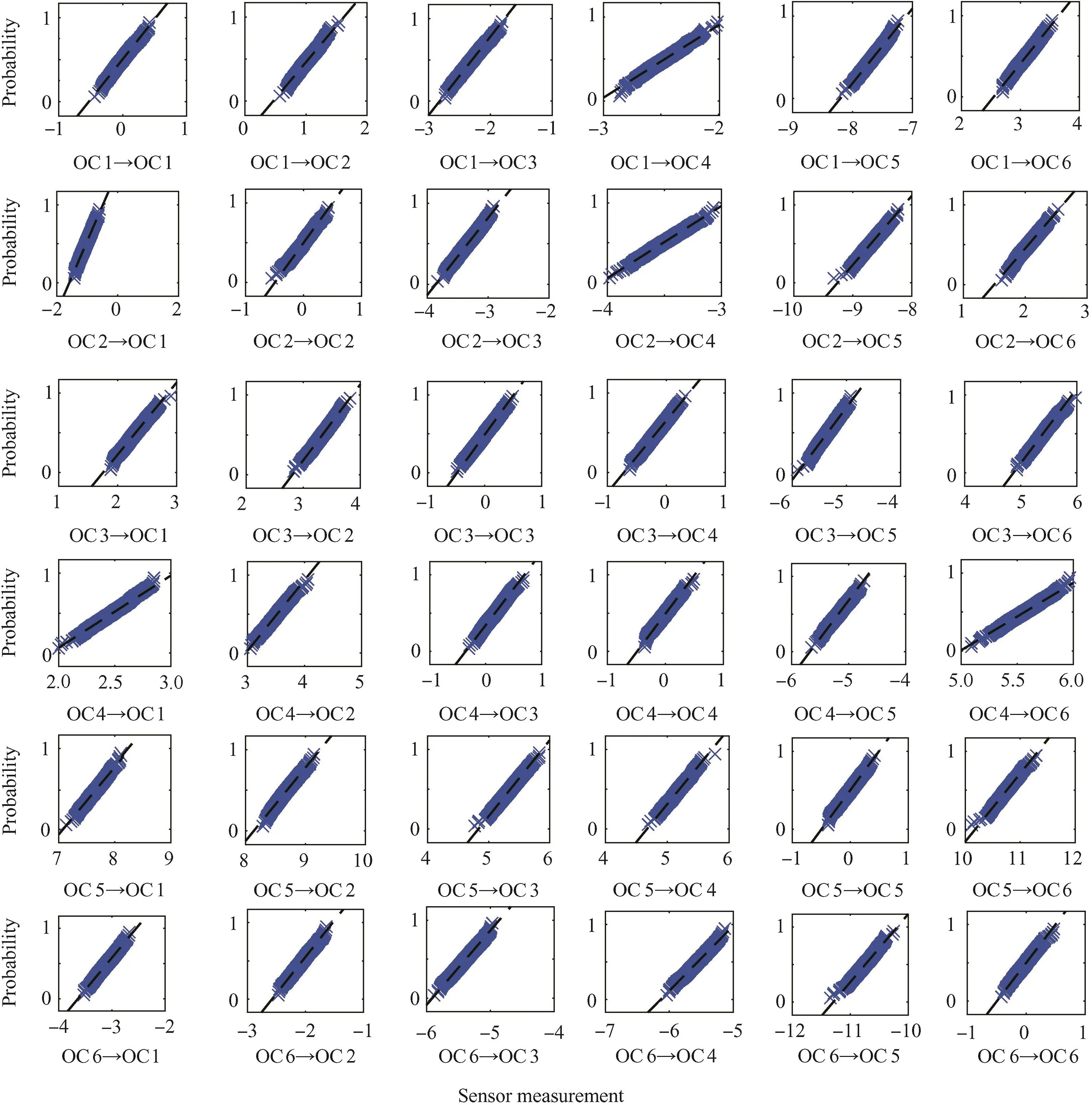
Fig.7 Normal probability plots for 36 elements in G11for Sensor 11.

Because each simulated path{Z(n):nclt;n≤N}can be treated as a single,deterministic transition process of operational conditions,RUL can then be estimated based on each path independently.Subsequently,applying the law of large numbers,the expected mean RUL can be obtained by averaging RULs of all sample paths.The estimation procedure is detailed as follows:

Step 1.Set the largest possible lifetime N(cycles)and the number of sample paths to simulate, M (e.g.,M=100000).For this dataset,since the longest lifetime found in training data set is 357,we assume N=400.

Step 2.Select any Sensor s from candidate sensorsconstruct its failure zones by the method proposed in Section 3.2,and develop its degradation model according to the model described in Section 4.

Step 3.For each Unitlin the testing dataset,if the unit's latest sensor measurement is observed at tnc=nch,we simulate M sample paths of the operational conditions' future evolution for the time interval[(nc+1)h,Nh]according to the limiting probabilities in Table 3,given the operational condition Z(nc)at time tnc=nch.Here we define tnc=nch as the prediction starting point.

Step 4.Use a specific sample path p(p=1,2,...,M)simulated from Step 3 to calculate the expected degradation state E[Ys(n)]at each cycle time tn=nh by Eq.(9),and then identify RUL according to different operational condition k,k∈C.Here RUL is determined by the first entering time of the failure zone:

Step 5.For systems requiring stringent reliability(e.g.,aircraft engine),the situation that the estimated RUL is less than the true RUL is better than the situation that the estimated RUL is larger than the true RUL;therefore,it is necessary to remove overlarge RULs.For this dataset,since the largest lifetime in the training dataset is 357 cycles,we remove those estimation RULs that are larger than 360-tnc.

Step 6.Since sensor measurements may have been contaminated by noise,using more sensor measurements to reduce the possibility of random error is very likely to bene fit the final result.Take b time epochsprior to tnc=nch as other prediction starting points,and repeat Steps 3–5 to estimatewhere i=0,1,...,b,then the estimatedis combined by the weighted average of all

where ωiis determined by how reliable the sensor measurement at time tnc-i=(nc-i)h is,and I(i)is the indicator function which equals to 0 whenis larger than 360-tnc-i,and equals to 1 otherwise.In this paper,we consider the same value for each ωi.

Step 7.For a sufficiently large integer M,RUL for Unitlestimated by sensor measurements of Sensor s is given by

Step 8.Select another sensor and repeat Steps 2–6.

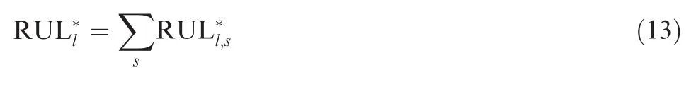
Step 9.Obtain the final resultfor testing unitlby averaging allof candidate sensors,which is given by

5.2.RUL estimation results

Following the steps in Section 5.1,we are able to estimatebased on sensor measurements of each sensor s for each testing unit l,and a more accuratecan be achieved by combining all results of candidate sensors.Table 4 lists the evaluation results for allandusing the evaluation metrics de fined in Section 2.1,and it shows that:

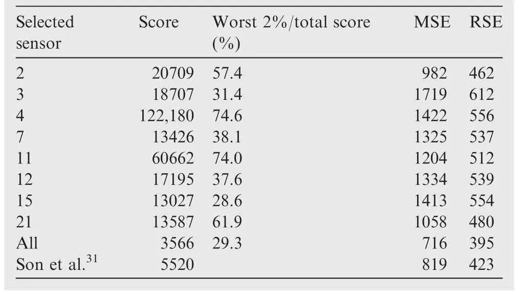
Table 4 Evaluation of RUL estimation results for 218 testing units.

(1)Although single sensor is not able to possess competitive prognostic abilities,the prediction performance can be greatly improved by combining the results of all candidate sensors in.Compared with the probabilistic method proposed by Son et al.,31our probabilistic method shows a superior performance by lower Score,MSE and RSE.Moreover,comparison with nonprobabilistic methods including similarity method(Score=563628) and neural network methods(MSE=98429,RSE=519.830)also reveals the effectiveness of the proposed method.

(2)If the prediction accuracy(MSE or RSE)is the only evaluation metric,the results using single sensor are kind of acceptable.Especially,MSE and RSE using Sensor 2 are very close to their counterparts in the study of Son et al.,31which used 7 sensors(Sensors 2,3,4,7,11,12,15)in the prediction.This phenomenon reflects that our degradation features and degradation model more accurately describe the degradation process of this dataset.However,due to possible noises contained in the sensor measurements,the results of each sensor are better to be combined in order to provide a better performance.

(3)The worst 5 predictions(2%of the total units)contribute a relatively huge amount to the total Score,which means if special cases can be clearly located and appropriately dealt with,the prediction performance is very likely to be improved.

5.3.Optimization of sensor set

Not only does our method present a better performance compared with the existing benchmark methods,it also enables the possibility of reducing the number of involved sensors without losing any prediction accuracy.Among all existing methods for this dataset,some methods28,31proposed to use the sensor set{2,3,4,7,11,12,15},and some methods used the whole 21 sensors.29,30Since their methods depend on virtual health indicators,their sensor sets cannot be further truncated after the degradation model is developed.Moreover,as we have mentioned in Section 2.1,some sensors do not contain much degradation information or have too much noise,so including them may even lower the prediction accuracy.

In this section,an optimization procedure using k-fold cross validation(CV)is proposed to find the optimal sensor set.The procedure calculates the CV error for each candidate sensor set and determines the optimal sensor set by the lowest CV error.It randomly divides the original training dataset into k mutually exclusive subsets.Each subset has an approximately equal size.Of the k subsets,one is used as the testing set and the other k-1 subsets are put together as a training set.The samples in the training set contain the complete degradation information while the ones in the testing set carry only partial degradation information.The latter is achieved by randomly right-censoring the complete degradation information.The CV process executes k times,with each of the k subsets used exactly once as the testing set.Then the CV error is computed as the average error over all k trials and can be expressed as

Table 5 Results of optimal sensor sets and their prediction performance.

When we apply the above method to our case,the 218 training units are divided into 10 subsets with similar sizes.We use two evaluation metrics,Score and MSE,to calculate CV errors,and to find the optimal sensor set under each constraint of pre-determined number of sensors.The results are listed in Table 5.The optimal sensor sets are tested by the testing dataset,and their prediction performances are shown in Table 5 as well.

In Table 5,we notice that increasing the number of sensors do not necessarily improve the prediction performance.For example,four sensors or five sensors seem to be less efficient than two sensors.This is an important discovery emphasizing the significance of using quantitative methods to select the most useful data sources while making RUL estimations.We also notice from Tables 4 and 5 that the prediction performance by combining all candidate sensors'results is possibly less satisfactory than that by combining part of all results.As the Score,MSE and RSE show,the prediction results by six sensors or seven sensors are better than those by all eight candidate sensors

In Table 5,the best prediction result for the testing dataset is obtained by the sensor set{2,3,4,11,15,21},and the result is Score=3120,MSE=639 and RSE=373.We also calculate Score,MSE and RSE using sensor set{2,3,4,7,11,12,15},which is most commonly used in the existing methods28,31,and the results are Score=3509,MSE=707 and RSE=392.This comparison indicates that different RUL estimation methods may have to carefully select their data sources in order to achieve a higher accuracy.

We plot in Fig.8 all RUL estimation results for the testing unit using single Sensor 15 and the results using the sensor set{2,3,4,11,15,21},respectively.Although the results using single Sensor 15 obtain the lowest Score among all single sensors(Table 4),from Fig.8 we can observe that these RUL estimations have too much advancing predictions.This situation can be greatly improved by combining results of more sensors.

Fig.8 RUL estimation results for 218 testing units.

Fig.8 gives an example of how multiple sensors efficiently improve the prediction performance.

6.Conclusions

(1)A RUL estimation method for deteriorating systems with dynamic time-varying operational conditions and condition-specific failure zones is proposed in this paper.The method deals with the periodically monitored degrading systems,and instead of eliminating the difference caused by different operational conditions,it quantifies those differences according to different operational conditions and different transitions of operational conditions.

(2)The 2008 PHM Conference Challenge Data is utilized in this paper as an illustrative example,and through it we develop a complete RUL estimation procedure including selection of sensors which relate to the underlying degradation process,construction of different failure zones,development of the degradation model,RUL estimation method and optimization of the sensor set.The description of this procedure usually comes with necessary statistical analysis,providing the tools to validate the approaches while implementing this proposed method to different problems.

(3)One uniqueness of the proposed method is that under periodically monitored situation,the dynamic process of time-varying operational conditions is assumed to evolve as a DTMC,and the degradation model is simplified by assuming that the transition of different operational conditions is the main factor to affect the degradation process,which allows us to quantify degradation increments by probabilistic approaches according to operational conditions at adjacent monitoring epochs.

(4)The second uniqueness is that the failure thresholds are determined by specific operational conditions and are described as different failure zones,thus we develop RUL estimation method through a path averaging approach which simulates a large number of samples of the operational condition's future evolution.

(5)As a probabilistic method,our method shows a more satisfactory performance compared with the existing probabilistic method(Son et al.31)for this dataset,demonstrating the advantages of differentiating the effects of different operational conditions.

This work explores the great potential of excavating the effect of different operational conditions on degradation process and prognostics,and inspires more future research topics regarding the prognostics under dynamic operational conditions.Since only 8 sensors are included in our current method,how to extract degradation information from more sensors in order to strengthen the prediction accuracy thus deserves further study.Besides,we only consider degradation systems subject to discrete monitoring at equidistant cycle epochs;however,situations with different monitoring strategies can be discussed further.Another interesting future research could be the development of appropriate model updating approaches to enable the model's ability of fitting different individuals.

Acknowledgement

This study was supported by the Fundamental Research Funds for the Central Universities(No.YWF-14-ZDHXY-16).

1.Lu CJ,Meeker WO.Using degradation measures to estimate a time-to-failure distribution.Technometrics 1993;35(2):161–74.

2.Chinnam RB.On-line reliability estimation for individual components using statistical degradation signal models.Qual Reliab Eng Int 2002;18(1):53–73.

3.Tang DY,Makis V,Jafari L,Yu JS.Optimal maintenance policy and residual life estimation for a slowly degrading system subject to condition monitoring.Reliab Eng Syst Saf 2015;134:198–207.

4.Tang DY,Yu JS,Chen XZ,Makis V.An optimal condition-based maintenance policy for a degrading system subject to the competing risks of soft and hard failure.Comput Ind Eng 2015;83:100–10.

5.Wang X.Wiener processes with random effects for degradation data.J Multivariate Anal 2010;101(2):340–51.

6.Gebraeel NZ,Lawley MA,Li R,Ryan JK.Residual-life distributions from component degradation signals:a Bayesian approach.IIE Trans 2005;37(6):543–57.

7.Si XS,Wang WB,Hu CH,Chen MY,Zhou DH.A Wiener process-based degradation model with a recursive filter algorithm for remaining useful life estimation.Mech Syst Signal Process 2013;35(1):219–37.

8.Wang HW,Xu TX,Mi QL.Lifetime prediction based on Gamma processes from accelerated degradation data.Chin J Aeronaut 2015;28(1):172–9.

9.Lawless J,Crowder M.Covariates and random effects in a Gamma process model with application to degradation and failure.Lifetime Data Anal 2004;10(3):213–27.

10.Wang X,Xu D.An inverse Gaussian process model for degradation data.Technometrics 2010;52(2):188–97.

11.Ye ZS,Chen N.The inverse Gaussian process as a degradation model.Technometrics 2014;56(3):302–11.

12.Elwany AH,Gebraeel NZ,Maillart LM.Structured replacement policies for components with complex degradation processes and dedicated sensors.Oper Res 2011;59(3):684–95.

13.Bian L,Gebraeel N.Computing and updating the first-passage time distribution for randomly evolving degradation signals.IIE Trans 2012;44(11):974–87.

14.You MY,Liu F,Wang W,Meng GA.Statistically planned and individually improved predictive maintenance management for continuously monitored degrading systems.IEEE Trans Reliab 2010;59(4):744–53.

15.Si XS,Wang WB,Chen MY,Hu CH,Zhou DH.A degradation path-dependent approach for remaining useful life estimation with an exact and closed-form solution.Eur J Oper Res 2013;226(1):53–66.

16.Si XS.An adaptive prognostic approach via nonlinear degradation modeling:application to battery data.IEEE Trans Ind Electron 2015;68(8):5082–96.

17.Chen XZ,Yu JS,Tang DY,Wang YX.A novel PF-LSSVR-based framework for failure prognosis of nonlinear systems with time varying parameters.Chin J Aeronaut 2012;25(5):715–24.

18.Bian L,Gebraeel N,Kharoufeh JP.Degradation modeling for real-time estimation of residual lifetimes in dynamic environments.IIE Trans 2015;47(5):471–86.

19.Zhang JX,Hu CH,Si XS,Zhou ZJ,Du DB.Remaining useful life estimation for systems with time-varying mean and variance of degradation processes.Qual Reliab Eng Int 2014;30(6):829–41.

20.Guo YY,Jiang B,Zhang YM,Wang JF.Novel robust fault diagnosis method for flight control systems.J Syst Eng Electron 2008;19(5):1017–23.

21.Bu S,Yu F,Liu P.Stochastic unit commitment in smart grid communications.IEEE INFOCOM 2011 workshop on green communications and networking;2011 Apr 10–15;Shanghai,China.Piscataway(NJ):IEEE;2011.p.307–2.

22.Liao H,Tian Z.A framework for predicting the remaining useful life of a single unit under time-varying operating conditions.IIE Trans 2013;45(9):964–80.

23.Bian L,Gebraeel N.Stochastic methodology for prognostics under continuously varying environmental profiles.Stat Anal Data Min 2013;6(3):260–70.

24.Kharoufeh JP,Cox SM.Stochastic models for degradation-based reliability.IIE Trans 2005;37(6):533–42.

25.Kharoufeh JP,Solo CJ,Ulukus MY.Semi-Markov models for degradation-based reliability.IIE Trans 2010;42(8):599–612.

26.Si XS,Hu CH,Kong XY,Zhou DH.A residual storage life prediction approach for systems with operation state switches.IEEE Trans Ind Electron 2014;61(11):6304–15.

27.Saxena A,Goebel K.Turbofan engine degradation simulation dataset Internet;2008[2013-09-12].Available from:http://ti.arc.nasa.gov/tech/dash/pcoe/prognostic-data-repository/.

28.Wang TY,Yu JB,Siegel D,Lee J.A similarity-based prognostics approach for remaining useful life estimation of engineered systems.Proceedings of the 2008 international conference on prognostics and health management;2008 Oct 6–9;Denver,(CO).Piscataway(NJ):IEEE;2008.

29.Heimes FO.Recurrent neural networks for remaining useful life estimation.Proceedings of the 2008 international conference on prognostics and health management;2008 Oct 6–9;Denver(CO).Piscataway(NJ):IEEE;2008.

30.Peel L.Data driven prognostics using a Kalman filter ensemble of neural network models.Proceedings of the 2008 international conference on prognostics and health management;2008 Oct 6–9;Denver(CO).Piscataway(NJ):IEEE;2008.

31.Son KL,Fouladirad M,Barros A,Levrat E,Lung B.Remaining useful life estimation based on stochastic deterioration models:A comparative study.Reliab Eng Syst Saf 2013;112:165–75.

32.Wang TY.Trajectory similarity based prediction for remaining useful life estimation dissertation.Cincinnati(OH):University of Cincinnati;2010.p.32–4.

33.Saxena A,Goebel K,Simon D,Eklund N.Damage propagation modeling for aircraft engine run-to-failure simulation.Proceedings of the 2008 international conference on prognostics and health management;2008 Oct 6–9;Denver(CO).Piscataway(NJ):IEEE;2008.

34.Saha B,Goebel K,Poll S,Christophersen J.Prognostics methods for battery health monitoring using a Bayesian framework.IEEE Trans Instrum Meas 2009;58(2):291–6.

Li Qiis a Master student in School of Automation Science and Electrical Engineering at Beihang University,Beijing,China.She received her Bachelor degree in measurement control technology and instruments from Beijing Jiaotong University in 2013.Her main research interests are prognostic and health management and remaining useful life estimation.

Gao Zhanbaois a lecturer in School of Automation Science and Electrical Engineering at Beihang University,Beijing,China.He received his Ph.D.degree from the same university in 2006.His current research interests are prognostic and health management and remaining useful life estimation.

Tang Diyinreceived her Bachelor and Ph.D.degrees from Beihang University,Beijing,China in 2008 and 2015,respectively.From 2012 to 2013,she was a visiting Ph.D.student in Department of Mechanical and Industrial Engineering at University of Toronto,Canada.She is currently a lecturer in School of Automation Science and Electrical Engineering at Beihang University,Beijing,China.Her research interests are condition-based maintenance,fault diagnostics,and failure prognostics.

Li Baoanis an associate professor in School of Automation Science and Electrical Engineering at Beihang University,Beijing,China.He received his Ph.D.degree from the same university in 2002.His current research interests are prognostic and health management and flight safety of UAV.

8 July 2015;revised 18 November 2015;accepted 13 January 2016

Available online 9 May 2016

Degradation;

Discrete-time Markov chain;

Operational conditions;

Remaining useful life estimation;

Sensor selection

?2016 Chinese Society of Aeronautics and Astronautics.Production and hosting by Elsevier Ltd.This is an open access article under the CCBY-NC-ND license(http://creativecommons.org/licenses/by-nc-nd/4.0/).

*Corresponding author.Tel.:+86 10 82338693.

E-mail addresses:15210585903@163.com(Q.Li),gaozhanbao@buaa.edu.cn(Z.Gao),tangdiyin@buaa.edu.cn(D.Tang),superlba@163.com(B.Li).

Peer review under responsibility of Editorial Committee of CJA.