POD Applied to Numerical Study of Unsteady Flow Inside Lid-driven Cavity

Lucas Lestandi,Swagata Bhaumik,Tapan K Sengupta,G.R.Krishna Chand Avatarand Mejdi Aza¨?ez

1University of Bordeaux,I2M UMR 5295,France.

2High Performance Computing Laboratory,IIT Kanpur,Kanpur 22650,India.

3Bordeaux Institut National Polytechnique,I2M UMR 5295,France.

Abstract.Flow inside alid-drivencavity(LDC)is studied hereto elucidatebifurcation sequences of the flow at super-critical Reynolds numbers(Recr1)with the help of analyzing the time series at most energetic points in the flow domain.The implication of Recr1in the context of directsimulation of Navier-Stokes equation is presentedhere for LDC,with or without explicit excitation inside the LDC.This is aided further by performing detailedenstrophy-basedproperorthogonal decomposition(POD)ofthe flow if eld.The flow has been computed by an accurate numerical method for two different uniform grids.POD of results of these two grids help us understand the receptivity aspects of the flow field,which give rise to the computed bifurcation sequences by understanding the similarity and differences of these two sets of computations.We show that POD modes help one understand the primary and secondary instabilities noted during the bifurcation sequences.

AMS subject classifications:65M12,65M15,65M60,76D05,76F20,76F65

Keywords:Lid drivencavity,POD,POD modes analysis,DNS,multiple Hopf bifurcation,polygonal core vortex.

1 Introduction

The 2D flow in a square LDC(of side L)is a canonical problem to study flow dynamics numerically for incompressible Navier-Stokes equation due to its unambiguous boundary conditions and very simple geometry.The flow is essentially shear-driven,with the lid given a constant-speed translation(U),giving rise to corner singularities on the top wall,as depicted in the top frame of Figure 1.Such singularity gives rise to Gibbs’phenomenon[1,5],which is milder for low order methods[16,29].Low order highly diffusive methods[6,16]are incapable of computing unsteady flows at high Reynolds number(Re=UL/ν,where ν is the kinematic viscosity).In Ghia et al.[16],results for a wide range of Re up to 10000 are presented as steady flow.However,numerical results obtained by high accuracy combined compact difference scheme indicate creation of a transient polygonal vortex at the core,with permanent gyrating satellite vortices around it[38,42],for the same Re.It is well known that compact schemes for spatial discretization behave properly as compared to other methods,and Gibbs’phenomenon[35]is not experienced for the singular LDC problem due to numerical smoothing of the derivatives near the Nyquist limit[31,39].

Steady solutions have been reported[14,16]for Re far exceeding the values reported in the literature for the first Hopf Bifurcation(Recr1).Unsteady flows have been obtained as a solution of bifurcation problem[26,43],by studying linear temporal instability of the steady solution obtained numerically.Simulations of full time-dependent Navier-Stokes equation[25,38]reveal that the flow loses stability via Hopf bifurcation,as Re increases.Critical Re and frequencies obtained from DNS and eigenvalue analysis do not match.Such differences are also noted for different DNS results.However,DNS approach is preferable,due to its superiority of spatio-temporal multi-modal analysis overnormal mode analysis of eigenvalue approach.In the latter,one postulatesexplicitly that all points in the domain have identical variation with respect to time.This is strictly incorrect,as one is dealing with space-time dependentgrowthof disturbances during the onset of unsteadiness.

It is shown[25,41,42]that Recr1depends upon accuracy of the method and how the flow is established in DNS.Impulsive start of the flow triggers all frequencies at the onset and hence preferred[38,42].Obtaining final limit cycle at one Re from the limit cycle solution from another Re[25]is inappropriate[22].First Hopf bifurcation obtained by DNS is dependent upon source of numerical error,mainly on the aliasing error for flow inside LDC[42].This also dependsupon the discretization,which in turn determines the creation of wall vorticity.A finer grid will create larger wall vorticity,but will have lesser truncation error.For the same numerical method,using same time step,a finer grid will have lesser aliasing and truncation errors,and hence numerical Recr1will be higher forfiner grid.However,this can also be studied with the help of explicit excitation to show the near universality of Recr1.

Linear instability of equilibrium flow and DNS have been used to evaluate the onset of unsteadiness,i.e.,obtaining Recr1for LDC.These methods yield values of Recr1differently.For example,Recr1=8018 in[2]and 8031.93 in[28]have been reported.Cazemier et al.[8]reported Recr1at 7972 using a finite volume method.In Bruneau and Saad[6],the critical Re is suggested to be in the range of 8000≤Recr1≤8050,obtained using a third order upwind finite difference scheme.The authors do not provide any bifurcation diagram to substantiate this observation.Sengupta et al.[41]have described multiple Hopf bifurcations,showing the first one at 7933 and the second at 8187,using uniform(257×257)grid,with these values obtained from the FFT of vorticity time series.Osada and Iwatsu[25]have identifi ed this value at 7987±2%,obtained using compact scheme on non-uniform(128×128)and(257×257)grids.However,the authors do not produce any evidence for grid independent data.Shen[44]reported Recr1in the range of 10000 to 10500 obtained using partial regularization of top-lid boundary conditions.Poliashenko and Aidun[26]on the other hand reported a value of Recr1=7763±2%using a commercial FEM package.Using the present method[41]with a(257×257)grid,a value of Recr1≈8665 has been reported by Lestandi et al.[22],for the case of no explicit excitation applied.A major difference is that computations for all the cases presented here have been performed following an impulsive start.

The point located at(x=0.95,y=0.95)is used here for sampling the data,which is very close to the singularity at the top right corner,and will log larger value of disturbances[22,41,42].A recent study[22]highlights aspects of computing flow inside LDC based on study of time series at this point.Although,it is a valid way of studying the flow dynamics in LDC,it is desirable to use a global flow analysis tool like POD,whichprovides spatio-temporalinformation forthe full domain.PODwas introducedby Kosambi[21]to project a stochastic field on to a finite set of deterministic basis functions in the most optimum way possible.POD is also known as Karhenen-Loeve decomposition,principal component analysis,etc.This method requires solving an optimization problem of variational calculus,whose discrete version is a linear algebraic eigenvalue problem that decomposes a stochastic field into a set of eigenfunctions.Once the eigenvalues and eigenfunctions are obtained,one can obtain the time dependent amplitude functions,which apportion disturbance field into different eigenmodes.

There are many versions of POD reported in the literature.The eigenvalues may be obtained through a variety of methods including direct[9]and iterative solvers such as a Lanczos procedure[34],with or without re-orthogonalization,as given by Cullum and Willoughby[10].One of the advantage is that this method can be used locally,in a small zone of investigation,with the number of eigenvalues depending on the total number of points in that small part of zone investigated.

However,even such a local analysis can be very resource-intensive.Thus,one uses instead the alternative method of snapshots proposed by Sirovich[45].In this case,the number of eigenvalues depends upon number of snapshots used for the investigation.The popularity of this method rests with the use of limited number of snapshots,thereby making the method very efficient.Like the classical method,the problem of optimization in projection used for method of snapshots also involves obtaining two-point correlation functions.POD with method of snapshots have been used in fl uid mechanics originally with the idea of applying it to turbulent flows[19],with the number of modes decided upon capturing a very high percentage of kinetic energy.This has been followed in many early attempts[8,11,23,24]to build POD based reduced order models(ROMs),where primitive variable formulations have been used to convert the governing PDEs into a set of coupled ODEs for the amplitude functions.In doing so,the pressure gradient terms are usually omitted.This is avoided in an alternative approach,where stream function-vorticity formulation is used for the governing 2D Navier-Stokes equation and the projection onto a deterministic basis is sought in capturing maximum enstrophy[33,34,36,37,40].This does not entail omission of pressure information,as vorticity transport equation is not directly coupled to pressure.Also,in this approach of using DNS,one directly obtains the amplitude functions up to the desired numbers with enhanced accuracy.This helped classifying POD modes based on the properties of the amplitude functions[40,41],in terms of regular and anomalous modes.In[40],the POD modes have been related with the instability modes for the first time,readying the field of flow instability study by POD analysis.The regular POD modes occur in pairs for the amplitude functions,separated by quarter cycle and the resultant instability modes obey the Stuart-Landau equation[30].The anomalous modes,on the other hand do not obey Stuart-Landau equation.Also,Stuart-Landau equation is of use for fl uid dynamic system with a single dominant mode.Hence,an augmented eigenfunction approach due to Eckhaus[13]has been used in instability studies of fl uid dynamic system with multiple modes.The resultant governing equations for instability modes have been termed as Stuart-Landau-Eckhaus equations.This approach of obtaining POD eigenfunctions and amplitude functions in describing nonlinear instability of fl uid flow has been described in[32]and is routinely used for incompressible flows[36,37].In[24],the authors devised a new POD mode which was obtained through a Galerkin projection on Reynolds-averaged Navier-Strokes(RANS)equation,and called it a shift mode.

Here,enstrophy is preferred over those in[19,24,27,45],where kinetic energy is used for POD analysis.In vortex dominated inhomogeneous flows,rotational energy is a better descriptor of POD over translational kinetic energy,as highlighted in[30,33,40].Authors in[41],used enstrophy based POD approach to study both external and internal flows to show universality of POD modes in terms of amplitude functions.

Thepaperis formattedin thefollowing manner.Inthenextsection,we providea very brief recap of the governing equation and numerical methods used.In Section 3,with the help of computed Navier-Stokes Equation(NSE)solution,we characterize the flow field by bifurcation analysis.POD as a tool has been used in Section 4,to relate vorticity dynamics in the LDC flow field about the sensitivity to grid resolution by solving NSE using two grids in describing primary and secondary instabilities.We close the paper by providing the conclusions arising out of this research.

2 Governing equations and numerical methods

Direct simulation of the 2D time-dependent flow is carried out by solving NSE in stream function-vorticity formulation given by,

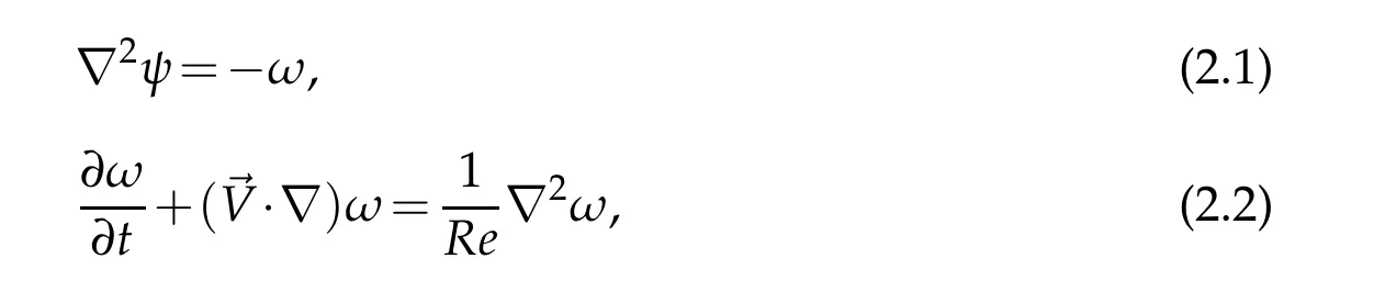
where ω is the only non-zero,out-of-plane component of vorticity for the 2D problem considered here.The velocity is related to the stream function as~V= ? ×~Ψ,where=[0,0,ψ]T.The governing equations are non-dimensionalized with L as the length scale and the constant lid velocity,(U),as the velocity scale,so that the Reynolds number is Re=.Consequently,computational domain is the unit square,while the time evolution is continued up to desired flow development.Present formulation is appropriate for 2D incompressible flows due to its inherent satisfaction of solenoidality condition for velocity and vorticity.This allows one to circumvent the pressure-velocity coupling problem,which is otherwise an important issue in primitive variable formulation.Identical numerical methods have been used previously of the flow for Re=10000 in[38,42]and is not repeated here.

Eqs.(2.1)and(2.2)are solved using uniform grid of a Cartesian frame with the origin at the bottom left corner of the LDC.A schematic of the computational domain is shown in Figure 1(a).The flow field is subjected to the following boundary conditions.On all the four walls of LDC,ψ=constant is prescribed,which satisfies no-slip condition and helps evaluating the wall vorticity as ωb= ?,with n as the wall-normal coordinate chosen for the four segments of the LDC.This is calculated using Taylor series expansion at the walls with appropriate velocity conditions on the boundary segments,as given for the top wall by,

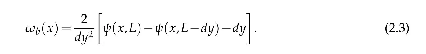
InEquation(2.3)ontheright hand side,the last termis dueto thetop lid continuously moving at the constant speed,U,which is taken equal to one in non-dimensional form.One can similarly obtain the expression for the wall vorticity at other wall-segments,where we use=0 identically.

To solve the discretized form of Eq.(2.1),Bi-CGSTAB method has been used here,which is a fast and convergent elliptic PDE solver[47].The convection and diffusion terms of Eq.(2.2)are discretized using the NCCD method[38,42]to obtain both first and second derivatives,simultaneously.For time advancing Equation(2.2)four-stage,fourth-order Runge-Kutta(RK4)method is used,that is tuned to preserve physical dispersion relation.The NCCD scheme has been analyzed for resolution and effectiveness in discretizing diffusion terms[38,42].It is noted that the NCCD scheme is particularly efficient,providing high resolution and effective diffusion discretization,as also has been shown with the help of model convection-diffusion equation[46].Additionally,it has built-in ability to control aliasing error.The only drawback of NCCD scheme is that it can be used only with uniform structured grids.All computations are performed with non-dimensional time-step of?t=10?3.Additional details of the method for this problem is in[22],which explained the reason for the location where time-series for vorticity is stored for analysis.This is shown in Figure 1(a)as P,with the coordinate(x=0.95,y=0.95).

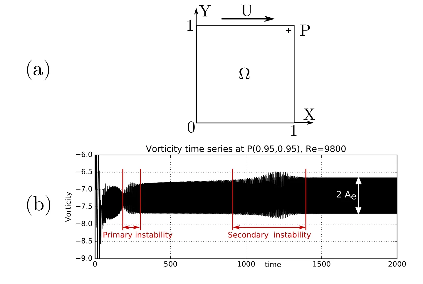
Figure 1:(a)Schematic view of the LDC problem and(b)time series of the vorticity taken at point P(0.95,0.95)obtained using(257×257)grid points for Re=9800.

3 Flow dynamics in LDC:Bifurcation sequences

To understand how a steady flow inside the LDC becomes unsteady with increasing Re above critical value,we record the time variation of the vorticity in the domain at point P,as shown in Figure 1(b).This is a typical time series,when we use the uniform grid with(257×257)points,for Re=9800 with the flow unexcited.

The used combined compact difference(CCD)scheme has near-spectral accuracy and it has been explained in[38,42],the onset of unsteadiness is due to aliasing error predominant near the top right corner of the LDC,while the truncation,round-off and dispersion errors are extremely negligible.To avoid the issue of lower numerical excitation in the present work[38,41,42],a pulsating vortex is placed having the form at r0=(0.015625,0.984375)whose spread is defined by α=0.0221 as given in the following,where in the presented results here we have taken f0=0.41 for different amplitude cases.

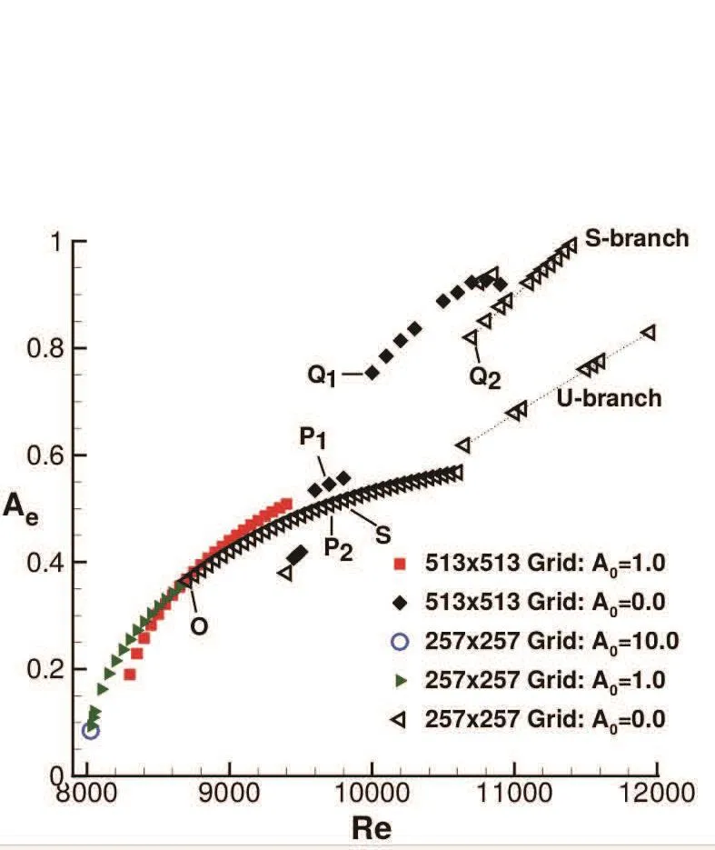
Figure 2:Variation of the equilibrium amplitude(Ae)with Reynolds number(Re)for the two grids,with(257×257)and(513×513)points.Note the points(P1,P2)and(Q1,Q2)have similar dynamics,as shown later.Additional points O and S represent the onset of unsteadiness(Re=8670)and secondary instability(Re=9800)of the flow field computed using(257×257)grid points.

From Figure 1(b)one notices a primary instability as marked in the frame,following subsidence of the initial transient.After this instability,one notices a regular time variation of vorticity(almost like a limit cycle,with slowly increasing amplitude).However,after some time,one notices rapidly growing envelope amplitude,caused by a secondary instability,following which one notes a final stable limit cycle,settling down to an equilibrium peak to peak amplitude indicated as 2Ae.

Figure 2 shows the variation of the equilibrium amplitude Aewith Re,for simulations performed using two grids,with(257×257)and(513×513)points.The triangles correspond to the equilibrium amplitude obtained using(257×257)grid points,except the highest amplitude case of A0=10 for this grid with open circle,for the lowest supercritical case.It shows the onset of unsteadiness for this grid to occur between Re=8660 and 8670 for the case of A0=0,with the point marked as ’O’in the figure.The points shown by filled rhombus and square are obtained using the(513×513)-grid points.For the refined grid,onset of unsteadiness occurs for Re slightly lower than 9450,for the case of A0=0.The(257×257)grid results also show a dip in Aearound Re=9400,which is identifi ed as the second bifurcation point[22]for this grid.In this reference,different bifurcation sequences are identifi ed by plotting A2eversus Re and the segments are identifi ed by straight lines with different slope for the unexcited cases.This stems from the literature which identifi es bifurcation with disturbance amplitude evolution following Stuart-Landau equation[30]to occur quadratically with respect to Reynolds number.However,this equation is valid only if there is a single dominant mode for the distur-bance field.It is understood that for circular cylinder,presence of many POD modes and instability modes necessitates adoption of Stuart-Landau-Eckhaus(SLE)equation to account for multi-modal interactions[40],which show quadratic variation of disturbance with Re merely as an assumption.In Figure 2,for the coarser grid we have identifi ed ’S’as the point(Re=9800)displaying secondary instability,as already shown in Figure 1(b).

For the finer grid,we note that the primary Hopf-bifurcation between Re=8660 and 8670 is bypassed.For this grid,the second and third bifurcations occur for Re=9600 and 10000,respectively.Following the second bifurcation,we notice three data points with the middle one identifi ed as P1in Figure 2,which show similar variation as for the(257×257)grid over an extended range of Re.Later on,we compare a representative point at P2with P1.A similar qualitative variation betweenthe two grids are noted which originate in a sequence starting from Q1and Q2,which are also compared later.

Few of the distinctive features of Figure 2 are the following:(a)The used methods for space-time discretization are so accurate that the onset of unsteadiness in the flowfield is delayed,with finer grid.Even for(257×257)-grid,the onset is delayed up to Re=8670.This has beenexplained here by performing the computations for lower Re,with an excitation applied at a single point by a pulsating vortex,with frequency of excitation of 0.41,which is distinctly different from the natural Strouhal number on 0.43.More details about the excitation is given in[22].Following this process of excitation,one notices from Figure 2 that the critical Re for this case can be brought down to between 8020 and 8025.(b)For the finer grid of(513×513)points,the first critical Reynolds number is noted between 9400 and 9425,for the case of no excitation.With excitation this can be brought down to as low as Re=8250(as shown in the figure).(c)For Re above 10400 with the(257×257)-grid,one notices two branches of solution,as shown in the figure.The lower branch(marked as U-branch)is essentially unstable and the upper branch is the stable branch,named as the S-branch.Upon application of slightest perturbations,the solution on the U-branch jumps to the S-branch.

4 Proper orthogonal decomposition

4.1 Method overview

Here,we use the enstrophy-based POD,which is preferred over those in[19,24,45],where kinetic energy-based POD analysis have been performed.In vortex dominated flows,which are neither homogeneous nor periodic,rotationality is more important and enstrophy is a better descriptor of POD over translational kinetic energy,as has been used in[32,36,37,40,41].Authors in[41],used enstrophy based POD approach to study both external and internal flows to show universality of POD modes in terms of amplitude functions.In[24],the authors devised a reduced order model(ROM)that relied on POD mode and Galerkin projection of RANS solution.Thus,POD analysis is noted to be useful in studying internal and external flows of different kinds.

POD technique introduced among others by Kosambi[21]for a random field vi(~x,t),whereit is projectedontoasetofdeterministicvectors ?i(~x),sothath|(vi,?i)|2i/||?i||L2is maximum.The outer angular brackets signify time-averaging and inner brackets signify an inner product.The computation of ?i(~x)can be posed as an optimization problem in variational calculus,

The kernel of the above is the two-point correlation function,of the random field.It is noted[32]that classical Hilbert-Schmidt theory applies to flows with finite energy,and,therefore,denumerable in finite orthogonal POD modes can be computed.Furthermore,Hilbert-Schmidt theory is applicable for flow instabilities,as the disturbancefield derives its energy from the equilibrium flow.Disturbance vorticity field is thus,represented in POD formalism as

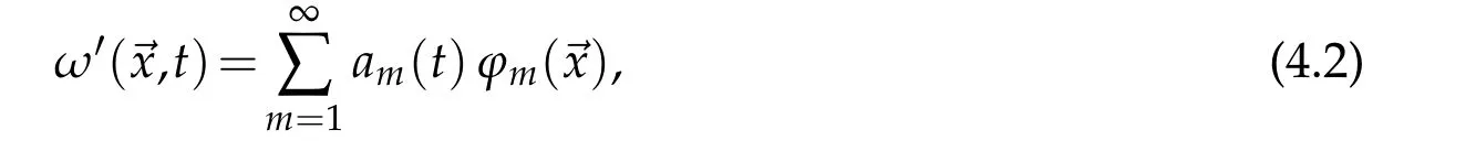
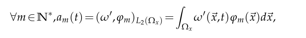
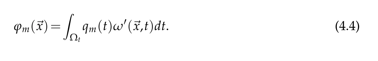
where am(t)representstheamplitude function,which describes the spatio-temporalvariation of the modal amplitude and ?m(~x)is the corresponding spatial eigenfunction.It should be noted that the eigenfunctions are orthogonal[9],additionally they are taken of unit norm for practical reasons.Thus,these form an orthonormal basis[3]on which ω′can be projected,as in Eq.(4.2).Then,one can compute the corresponding amplitude functions am(t)easily through spatial inner product

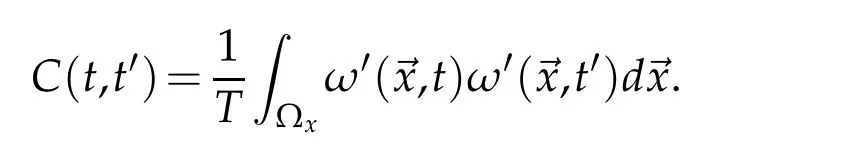
which emphasize the spatio-temporal nature of the POD.Equation(4.1)is an eigenvalue problem in the integral form,which becomes intractable even for moderate grid resolution.To overcome this difficulty,Sirovich[45]introduced the method of snapshots,which has an advantage of dealing with smaller data sets in multiple dimensions.Instead of solving Eq.(4.1),it is chosen to solve the equivalent problem on qmwhich yields the same decomposition,Z

where ?tis the time interval and the autocorrelation function is defined as

Once Eq.(2.2)has been solved,we can recover the spatial POD modes(?m)mdue to the following projection

Finally,(?m)are normalized and the norm is passed toThis method produces the same basis that one would obtain through classical POD.The strength of the snapshotPOD lies in the small size of the snapshotsof DNS data,where Ntthe numberof snapshots(time frames)that is lot smaller than the number of grid points NX.Discretization of the above operators is performed by trapezoidal integration rule for time(as well as space)with weights at time point i noted mi=dt/T,half of that for i=1 and i=Nt.The discrete version of the POD decomposition reduces to a simple matrix eigenvalue problem[]{q}=λ{q},where[]is given by

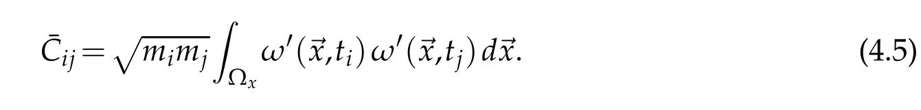
The eigenvalues λ and eigenvectors{q}of[ˉ]are computed using LAPACK eigenvalue problem solver for symmetric matrices(DSYEV).It should be noted that the calculations account for the differences between discrete L2inner product and vector scalar product.Consequently an extra step is required that reads qm=m?1{q}where m?i1=1/mi.

In this paper the maximum number of snapshots is Nt=1000 while the number of grid points is NX=66049 or 263169(according to grid size),thus only the method of snapshots is used.Moreover,the spatial POD modes will be referred to as eigenfunctions for historical reasons while(am)will be called amplitude function or time POD modes.

4.2 DNS data analysis:limit cycle

Here we use POD analysis to characterize flow fields obtained by the two grids.In Figure 3,the eigenfunctions obtained following the method of snapshots for the POD analysis is shown for the points,P1and P2,shown in Figure 2 for Re=9700.We display only the first twelve modes obtained for the two grids in Figures 3 and 4.It is noted that despite the differences in Figure 2 for the equilibrium amplitude and the associated maximum vorticity values in the domain,the first eight eigenfunctions have remarkable similarities,indicating the qualitative similarities of the associated flow fields obtained using two grids with significantly different points.The eigenfunction plots of Figures 3 and 4 also show a definitive pattern,with the first and second modes are regular modes[41],defined for classification of POD modes.In this case,one notices three pairs of similar vortical structures with opposite signs.In the same way,the third and fourth modes are composed of six such pairs;fifth and sixth modes similarly have nine pairs of structures.This multiplicity of vortical structures are extended to higher mode pairs also.However,their contributions are negligibly small in terms of enstrophy content,as the first eight modes in Figures 3 and 4,account for nearly all of the enstrophy contents for both the grids.

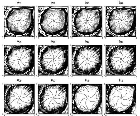
Figure 3:Eigenfunctions of POD modes for Re=9700 with(257×257)grid.These are for the two points(P1,P2)in Figure 2.(?m)misolines are plotted in the[?0.5,0.5]range with 0.01 spacing.Solid lines are positive values,while dashed lines are negative value contour. (Cont.)

Such similarities are furthermore emphasized in Figure 5,showing the cumulative enstrophyforthe pairing of pointsshownin Figure2.Forexample,in discussingthe flow dynamicsforpoints P1and P2,it hasbeenmentionedthatthe flowswouldbesimilar.This is clearly brought out in the eigenfunction plots of Figures 3 and 4 and the cumulative enstrophyshown in the top frames of Figure 5.Similarities for the points Q1and Q2have been suggested,while discussing the bifurcation diagram(Figure 2)and the cumulative enstrophyplot for this case showninthe bottomframe of Figure5,stronglysupportsthis.We also note that keeping the Reynolds number same with the two grids alone,does not ensure similarity of the flow,as noted from the cumulative enstrophy plot for Re=10000 in the middle frame of Figure 5.

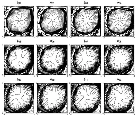
Figure 4:same modes with(513×513)grid points.

The POD amplitude functions,their representative DFT plots are shown in Figures 6 and 7 for Re=9700 case,obtained using the two grids.These are shown pairwise,when the two constituents differ by a phase shift of quarter cycle.In Figure 6,amplitude functions are shown for P1obtained using(513×513)grid.The FFT of these time series is shown in the bottom frames for each pair.The top left frame indicates the fundamental frequency for the first and second modes(f0=0.43),while the second,third and fourth mode pairs are the super-harmonics ofthis fundamental frequency(at 2f0,3f0,4f0).These amplitude functions and the frequencies are identical for both grids,as can be seen for the amplitude functions and their DFT shown for the point P2obtained using(257×257)grid.Once again the comparison betweenFigures 6 and 7 supportsthe view that the flow dynamics is similar for P1and P2.

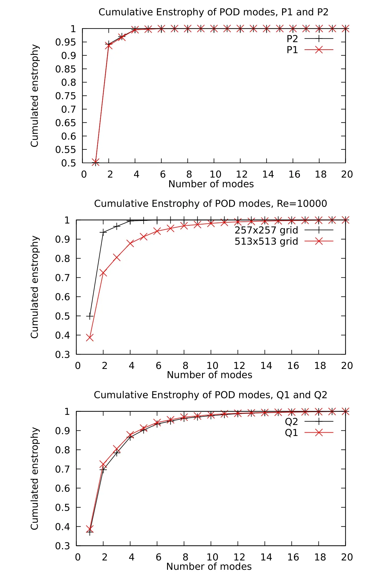
Figure 5:Cumulative enstrophy plots for the two grids shown for the indicated Reynolds number,for the enstrophy based POD.

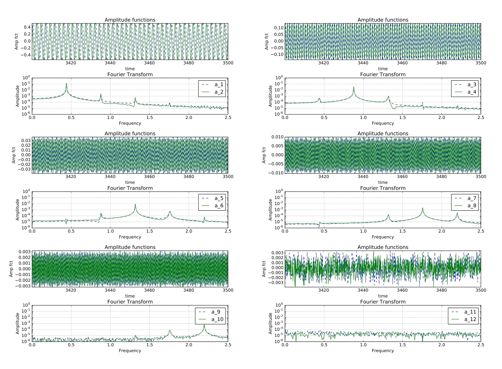
Figure 6:Amplitude of POD modes and its DFT for Re=9700 obtained for the(513×513)grid for the point P1in Figure 2.

Next,we investigate the flow fields for the points Q1(Re=10000)and Q2(Re=10700)of Figure 2,in Figures 8 and 9,respectively for the two grids with the help of POD eigenfunctions.Previously,we have noted that the flow fields for these points obtained by the two grids will be similar,while discussing the bifurcation diagrams in Figure 2.Now the plotted eigenfunctions for the first twelve modes in Figures 8 and 9 are also seen to be similar.This,added with the cumulative enstrophy plots shown in the bottom frame of Figure 5,strongly support the view that the flow fields are indeed similar.This also shows that the view provided by the bifurcation diagram is a better descriptor of similarity of flow field in the diagram,whenever A2eplotted against Re show identical slopes.The eigenfunctions have also similarity with the eigenfunctions shown in Figures 3 and 4 for the first two pairs,with respect to qualitative features.The higher modes are distinctly different in Figure 8 and 9,due to the flow fields belonging to different branches of the diagrams,as compared to the cases shown in Figures 3 and 4.Figures 8 and 9 belong to branches in which the instability is higher due to multiple dominant frequencies interacting[22].That causes the enstrophy to be distributed over larger number of modes,i.e.,one should be interested in the higher modes beyond the number eight,as was the case for the lower Reynolds number.Even the symmetry for the eigenfunctions noted for Re=9700 is lost from fifth mode onwards since two or more physical modes are interacting with the primary POD mode.

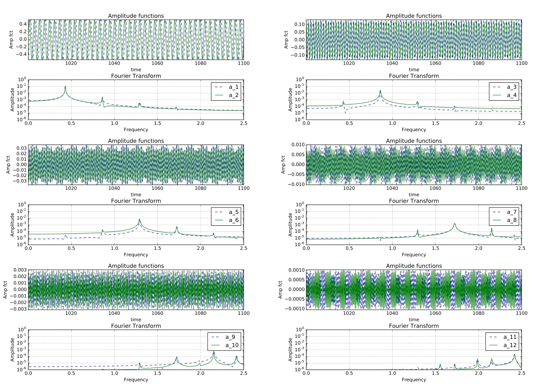
Figure 7:Amplitude of POD modes and its DFT for Re=9700 obtained for the(257×257)grid for the point P2in Figure 2.

The features of eigenfunctions for Q1and Q2are also re fl ected in the amplitude functions shown in Figures 10 and 11.The first pair of amplitude functions displays identical peak for these two grid results,which is different from the fundamental frequency(f0)noted in Figures 6 and 7 for Re=9800 case.The second pair of amplitude functions in Figures 10 and 11 are not the super-harmonic of the fundamental seen for the first pair of amplitude function.Thus,this segment of bifurcation diagram for Figures 10 and 11,is qualitatively different from the lower Reynolds number parts shown in Figures 6 and 7.Between the two points Q1and Q2,the third and fourth modes have some differences at the lower frequencies,otherwise other significant peaks are collocated.The fifth and sixth amplitude functions of POD modes again have the same value of frequency for the peak,as is notedfor the firstpair.All the othermodeshave qualitative similarity between amplitude functions for points Q1and Q2,and with the exceptionof eleventhand twelfth modes,all the modes appear as wave-packets,which have been called as the anomalous mode of second kind[30,41].

4.3 DNS data analysis:primary and secondary instabilities

So far,we have reported POD analysis of flow fields after the time series reaches stable limit cycle for the sampling point(x=0.95,y=0.95).We have previously reported DNS-based study of Hopf bifurcations using the(257×257)grid in[22],providing the numerical details of the methodology.Here we have studied the dynamics of the unsteady flow field using two different grids,with the intention of highlighting the mathematical physics of this canonical problem with POD as the analysis tool.It is necessary also to characterize the flow during primary and secondary instabilities.

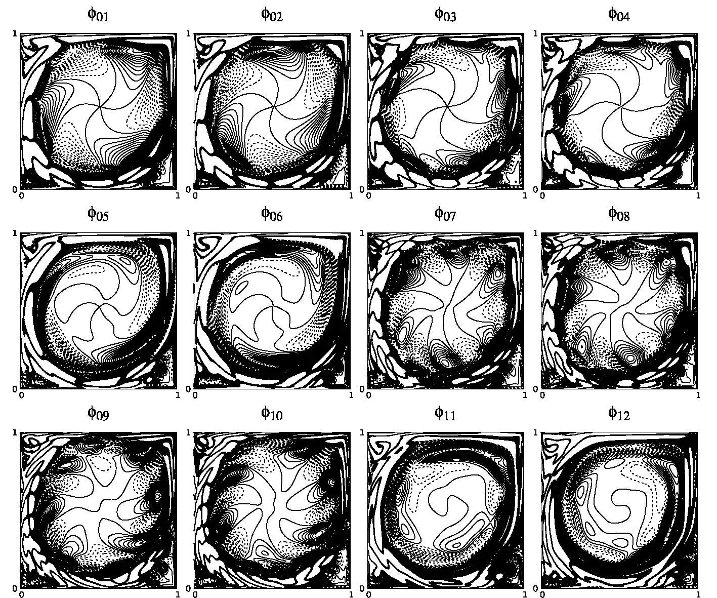
Figure 8:Eigenfunctions of POD modes for Re=10000 obtained with(513×513)grid for the point Q1in Figure 2.

For this purpose,in Figure 12 we show the POD eigenfunctions obtained without excitationduring theprimary instability stagefor Re=8670 obtainedusing the(257×257)grid,which is indicated as’O’inFigure 2.The first Hopfbifurcation obtained for this grid occurs between 8660 and 8670.Thus,this Re is a super-critical case that displays linear instability duringt=900 to1100.Theeigenfunctionsshowvariouspolygonalcore-vortex.For example,the eighth,fourteenth and seventeenth modes display triangular vortex at the core,as was shown for the flow field in[38,42]for Re=10000.Present simulation and its POD confirms the presence of triangular core vortex caused by the primary instability.

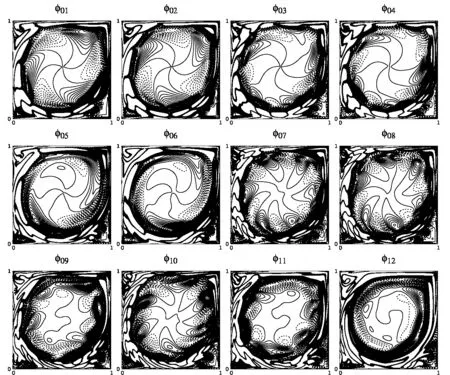
Figure 9:Eigenfunctions of POD modes for Re=10700 obtained with(257×257)grid for the point Q2in Figure 2.

This has also been advocated as the proof of accuracy of numerical schemes in[22],in capturing the triangular vortex at the core,as has been experimentally shown in[4,7,20].

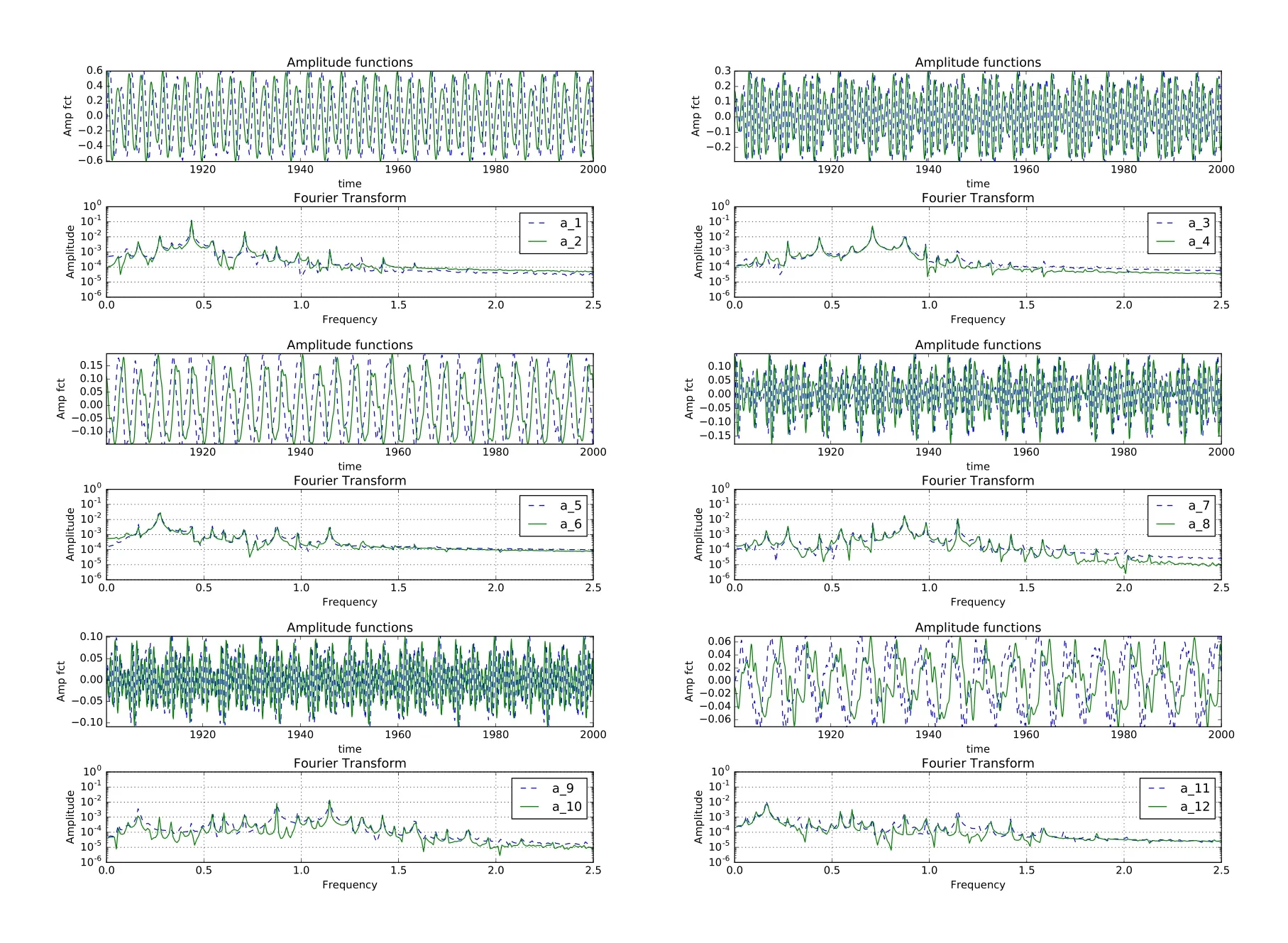
Figure 10:Amplitude of POD modes and its DFT for Re=10000 obtained for the(513×513)grid for the point Q1in Figure 2.

Forthe eigenfunctions shownin Figure 12 for Re=8670,the correspondingamplitude functions are shown in Figure 13.It is readily apparent that the first two modes form the regular pair[41],while the third mode is the anomalous mode of first kind;with fourth and fifth modes again form a regular pair,but modulated with higher frequency components.The sixth and seventh modes appear as wave-packets and hence,would be called the anomalous mode of second kind.The eighth and ninth modes are similar to fourth and fifth pair,i.e.,regular modes which are highly modulated.The tenth mode is an anomalous mode of first kind,similar to the third mode.It has been explained in[30,40]that the anomalous mode of first kind,gives rise to equivalent stress term,like the Reynolds stress and alters the mean flow.In this respect,the third and the tenth modes have opposite effects on the mean flow,as is evident from the signs of the amplitude at the terminal time.One can similarly classify the other modes into these categories described.However,the sixteenth and seventeenth modes appear as combination of the two types of anomalous modes described.It is worth remembering that the classification of POD modes like this is only feasible with DNS and not by RANS[24].Authors in this latter reference introduced the so-called shift mode,which possibly happen,if we time average the anomalous mode of the first kind using URANS approach.One of the features of the present approach is that one does not require performing time averaged computations using closure models.Anotherfeature of the anomalous mode of first kind is the appearance of the eigenfunctions in Figure 12,where one does not notice orbital motion of the vortices around the core,which gives rise to the polygonal vortex in the core.

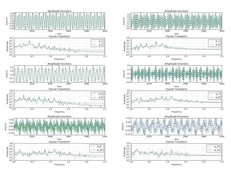
Figure 11:Amplitude of POD modes and its DFT for Re=10700 obtained for the(257×257)grid for the point Q2in Figure 2.

In describing the dynamics of LDC flow in real time plane in[22],it was noted that for some cases,limit cycle behaviour is noted after the primary instability(as characterized in Figure 12 and 13),but with slowly varying amplitude of the envelope.Such variations continue till a secondary instability occurs,following which a stable limit cycle is noted whose envelope does not change further with time.In the following,we report results of POD analysis of one such secondary instability noted for Re=9800,point’S’in Figure 2.The representative time series at(x=0.95,y=0.95)has been already shown in the bottom frame of Figure 1,marking the primary and secondary instabilities.In Figure 14(a)we show the eigenfunctions obtained by POD analysis performed on data before the beginning of secondary instability during t=500 to 600.At this stage,most of the enstrophy is contained in the first few modes and we show eight of these modes in Figure 14(a).One notices the onset of creation of the orbital vortices in the first six modes.The seventh mode is without any structure and is similar to the eigenfunction for the anomalous modes in Figure 12.It is the eighth mode that shows the appearance of a large triangular vortex in the core,with three pairs of orbital vortices surrounding the core.

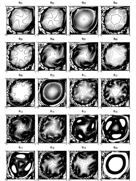
Figure 12:Eigenfunctions of POD modes for Re=8670 obtained with(257×257)grid for the point O in Figure 2 during the linear instability stage.

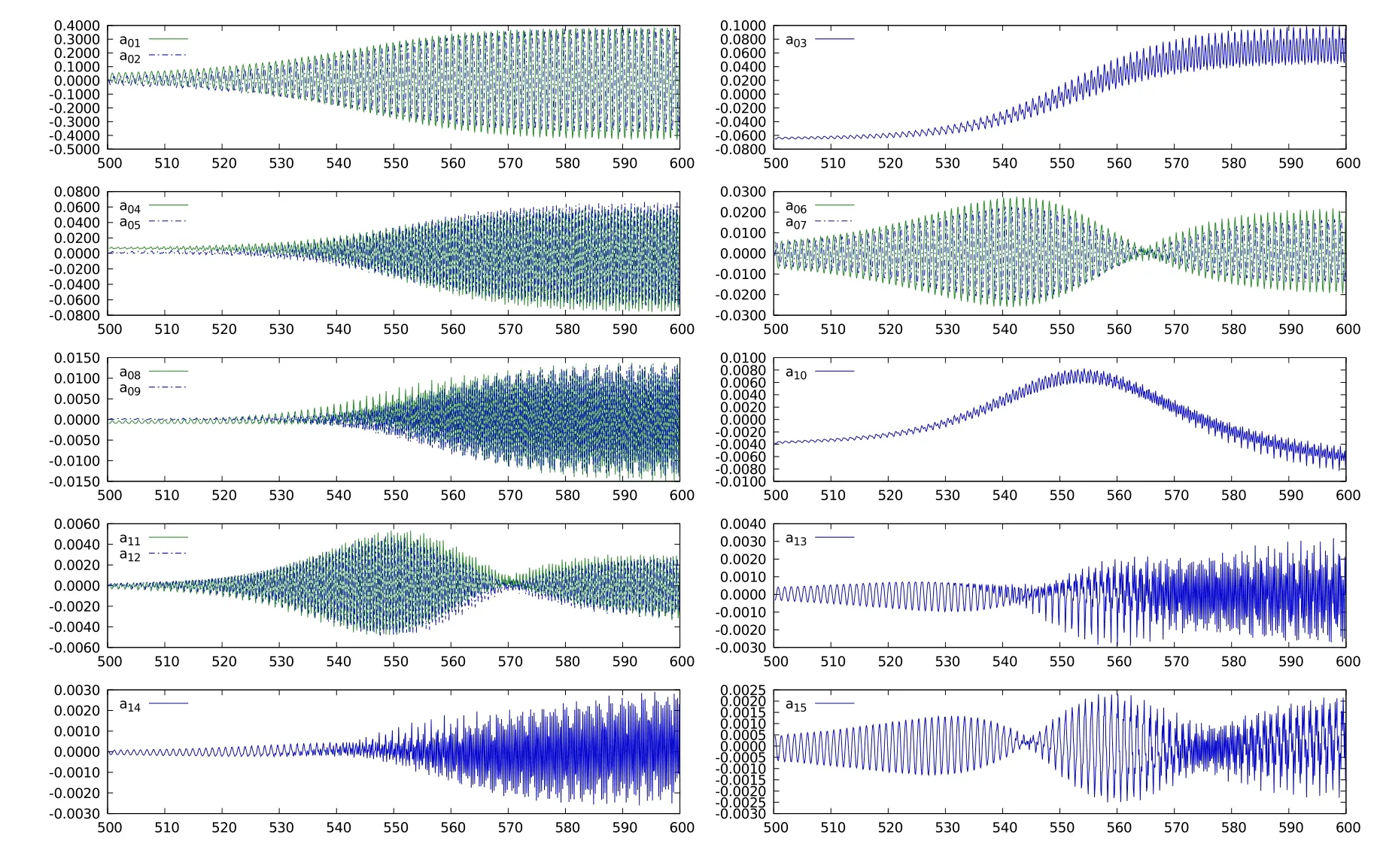
Figure 13:Amplitude of POD modes and its FFT for Re=10700 obtained for the(257×257)grid for the point Q2in Figure 2.

In Figure 14(b),we show the eigenfunctions for Re=9800 after the occurrence of the secondary instability during t=1900 to 2000.The first pair of eigenfunctions display three pairs of orbiting vortices,without any core vortex.This is typical of the behaviour of POD modes noted in the final limit cycle cases shown for higher Re.For the third and fourth modes,one notices six pairs of orbital vortices,without any core.The following two eigenmodes show nine pairs of orbital vortices and that is followed by the seventh and eighth modes,which show twelve pairs of orbital vortices.

The corresponding amplitudes and the DFT of various eigenmodes(as in Figure 14),are shown in Figure 15.In frames(a),the plotted amplitudes correspond to eigenfunctions shown in Figure 14(a),in pairwise fashion.One can clearly note that the FFT is dominated by a single mode and amplitudes are time-shifted by quarter cycle.While there is a distinct secondary mode,but its amplitude is orders of magnitude smaller.The third and fourth modes’amplitude shows the peak which has a value that is twice of that noted for the first pair.However,this mode-pair also shows modulation in the time plane,which is due to the secondary peak shown in the FFT,which is the fundamental for the first and second modes’amplitude.In the same way,the fifth and sixth modes have the peak at thrice the value noted for the first pair.The seventh and eighth modes have no correlation,as noted in Figure 15(a).

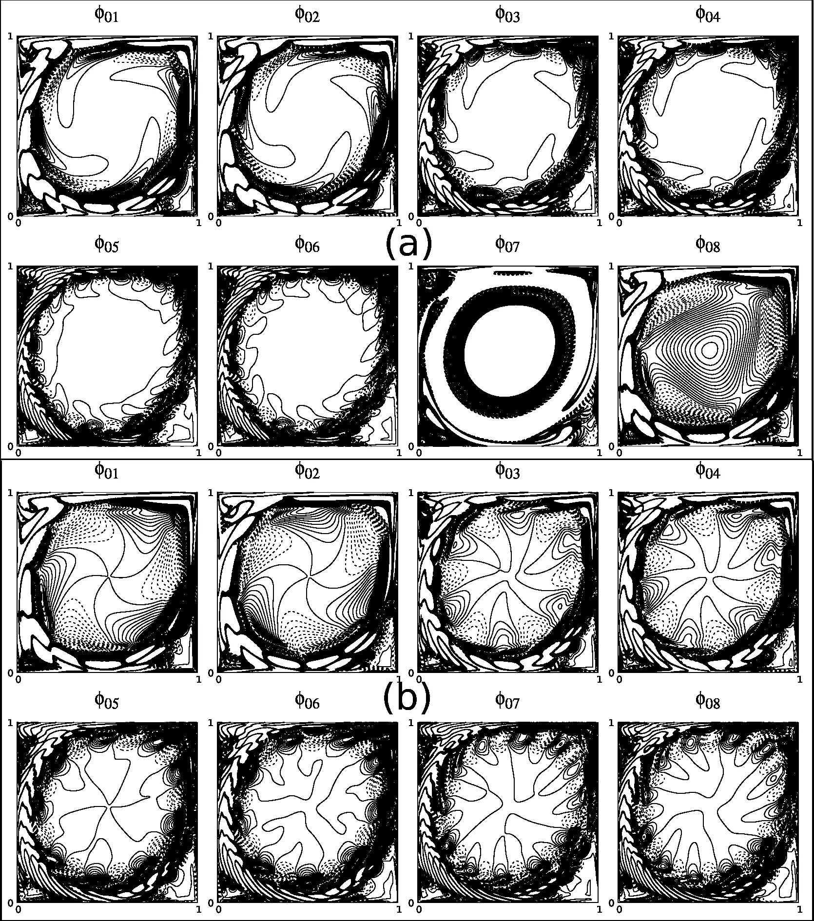
Figure 14:Eigenfunctions of POD modes for Re=9800 obtained with(257×257)grid during(a)t=500 to 600 before and during(b)t=1900 to 2000 after the secondary instability.

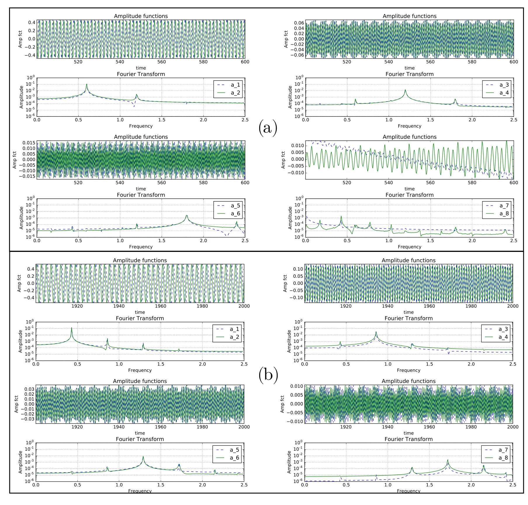
Figure 15:Amplitude of POD modes and its DFT for Re=9800 using(257×257)grid(a)before[t=500 to 600]and(b)after[t=1900 to 2000]the secondary instability,for the case of Figure 9.

In Figure 15(b),we note the amplitude functions corresponding to the eigenfunctions shown in Figure 14(b),obtained during t=1900 and 2000,when one is in the final limit cycle stage.It is interesting to note that the action of the secondary instability is to shift the fundamental frequency for the first pair((f0)before=0.60)to a lower value(f0=0.43),as noted in the FFT plots.The second and third pair of amplitude functions have peaks at 2f0and 3f0,respectively.The seventh and eighth modes are characterized by very high frequency fluctuations,and modulated at moderate frequencies,as a consequence one can categorize these as anomalous mode of second kind[41].This phenomenon is explained by similar amplitudes of the leading peak(4f0),with the next peak in amplitude(5f0)that interact to create modulations.This pattern is visible for each final state,however,it is weaker for the finer grid in Figures 3 and 4.

5 Conclusions

In the present research,we have used POD to characterize LDC flow for a range of Re for simulations performed using two grids(257×257)and(513×513)points.The numerical method is well established for similar exercise in[38,42],where very high accuracy combined compact scheme have been used.Although,the two grids produce different bifurcation sequences(in Figure 2),the reason for this is explained in exciting the flow,as determined by the aliasing error(which reduces with grid refinement),while the wall vorticity increases with the refined mesh.As a consequence,the relative scaled amplitude of disturbance field is lower for the finer mesh,and that also explains why primary Hopf bifurcation is delayed for the refined grid.Furthermore,we show that despite difference in bifurcation sequences in the two grids,the qualitative similarity of flow fields are noted for points in the bifurcation diagram.

We note that the flow is better characterized by the bifurcation diagram(Figure 2),rather than Re.The flow in the two grids will be similar when A2eversus Re curves have identical slope,even if the Re are different.This is shown first by comparing the POD modes of the flow field for Re=9700 for the two grids,which is expected from similarity of Re and the slope of the bifurcation diagram at P1and P2.The POD eigenmodes are shown in Fig.3 and corresponding FFT amplitude functions are shown in Fig.5 for P1and P2.This is also supported by comparing two points Q1and Q2in Fig.2,which correspond to Re=10000 using the(513×513)grid and Re=10700 for the(257×257)grid without excitation.The POD eigenfunctions and amplitudes together with FFT are shown in Figures 8–11.These observations are strongly supported by the cumulative enstrophy plots in Figure 5,for these four points,P1,P2,Q1and Q2.

We also characterize the primary temporal instability without excitation(indicated by point O in Figure 2)by POD analysis,showing eigenfunctions and amplitudes in Figures 12 and 13,which shows clearly multi-periodic dynamics of the flow,with a single dominant fundamental frequency and its super-harmonics.Finally,we characterize the secondary instability indicated in Figure 1 by showing POD eigenmodes and the corresponding amplitudes in Figs.14 and 15,during t=500 to 600 and then during t=1900 and 2000.These time intervals correspond to before and after the secondary instability for Re=9800,which has been identifi ed in Figure 1.We note that such secondary instability does not occur for all Reynolds number cases,but when it does occur,the effect is to change the fundamental frequency from a higher value(0.60)to a lower value(0.43).The eigenfunctions are also completely different,before and after the secondary instability.

This work reports the study of the LDC flow by DNS and resultant Hopf bifurcation patterns.The added understanding of this flow instability behaviour will allow us to build reduced order models relying on POD and the bifurcation diagram presented in Figure 2.It will focus on ranges of parameters for different ROMs,as we have shown that the nature of the flow changes drastically through Hopf bifurcation process.

Acknowledgements

The authors acknowledge the support provided to the first author from the Raman-Charpak Fellowship by CEFIPRA which made his visit to HPCL,IIT Kanpur possible.This work reports partly the results obtained during the visit.