
Chebyshev Spectral Method for Volterra Integral Equation with Multiple Delays
2018-08-06 06:10WeishanZhengandYanpingChen
Journal of Mathematical Study 2018年2期
Weishan Zhengand Yanping Chen
1College of Mathematics and Statistics,Hanshan Normal University,Chaozhou 521041,P.R.China;
2School of Mathematical Sciences,South China Normal University,Guangzhou 510631,P.R.China.
Abstract.Numerical analysis is carried out for the Volterra integral equation with multiple delays in this article.Firstly,we make two variable transformations.Then we use the Gauss quadrature formula to get the approximate solutions.And then with the Chebyshev spectral method,the Gronwall inequality and some relevant lemmas,a rigorous analysis is provided.The conclusion is that the numerical error decay exponentially in L∞ space and L2ωcspace.Finally,numerical examples are given to show the feasibility and effectiveness of the Chebyshev spectral method.
AMS subject classifications:65R20,45E05
Key words:Volterra integral equation,multiple delays,Chebyshev spectral method,Gronwall inequality,convergence analysis.
1 Introduction
In this paper,we consider the Volterra integral equation with multiple delays of the form
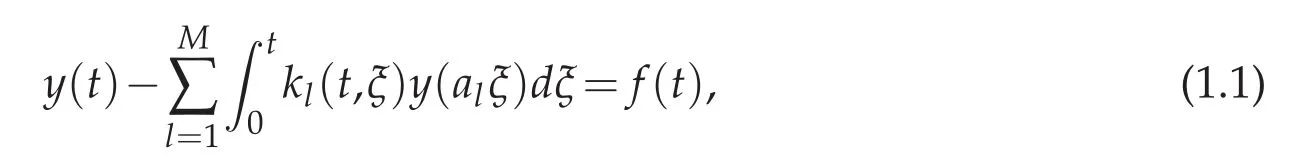
where the unknown function y(t)is defined on 0≤t≤T<+∞.The source function f(t)and kernel function kl(t,ξ)(l=1,2,...,M)are given sufficiently smooth functions,with the condition that M is a given natural number,0<al≤1.
These kinds of equations arise in many areas,such as the Mechanical problems of physics,the movement of celestial bodies problems of astronomy and the problem of biological population original state changes.It is also applied to network reservoir,storage system,material accumulation,etc.,and solve a lot problems from mathematical models of population statistics,viscoelastic materials and insurance abstracted.Due to the significance of these equations which have played in many disciplines,they must be solved efficiently with proper numerical approach.In recent years,these equations have been extensively researched,such as collocation methods[3–5,21],Taylor series methods[10],linear multistep methods[14],spectral analysis[1,2,7–9,11,18–20].In fact,spectral methods have excellent error properties called ”exponential convergence”which is the fastest possible.There are many also many spectral methods to solve Volterra integral equations,for example Legendre spectral-collocation method[18],Jacobi spectral-collocation method[8],spectral Galerkin method[20],Chebyshev spectral method[11]and so on.As the Chebyshev points are easier to be obtained than in[2],in this paper we are going to use the Chebyshev spectral method to deal with the Volterra integral equation with multiple delays.Meanwhile the error estimate of thenorm is observed in our article,while in I.Ali,H.Brunner and T.Tang′s is not.The third difference is that I.Ali,H.Brunner and T.Tang′s article only has two delay terms,while our article has M delay terms.Compared to the work by Zhang Ran in[22],the novelty is that the delay term in their article is in the integral term while in ours the delay terms are in the integrand functions.In a word,we provide rigorous error analysis by Chebyshev spectral method for the Volterra integral equation with multiple delays that theoretically justifies the spectral rate of convergence in this paper.Numerical tests are also presented to verify the theoretical result.
We organize this paper as follows.In Section 2,we introduce the Chebyshev spectral method.Some knowledge which is important for the derivation of the mail result is given in the next section.We carry out the convergence analysis in Section 4 and Section 5 contains numerical tests which are illustrated to confirm the theoretical result.In the end a conclusion is given in Section 6.
Throughout the paper C denotes a positive constant that is independent of N,but depends on other given conditions.
2 Chebyshev spectral method
In this section,we review Chebyshev spectral method.Firstly we use the variable transformations as follow
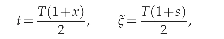
and if we note that

then(1.1)can be written as
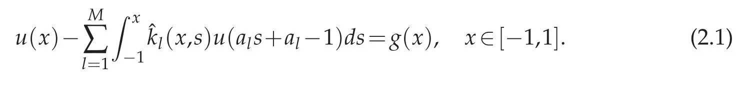
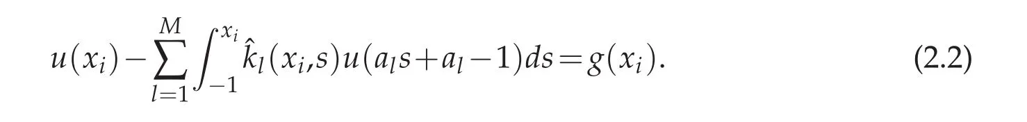
Set the collocation points as the set of N+1 Chebyshev Gauss,or Chebyshev Gauss-Radau,or Chebyshev Gauss-Lobatto points(see,e.g.,[6]).Assume that equation(2.1)hold at xi
The main difficulty in obtaining high order of accuracy is to compute the integral term in the above equation.Especially for small values of xi,there is little information useful for u(als+al?1).To overcome this difficulty,we transfer the integral interval into an fixed interval[?1,1]by the following simple linear transformation
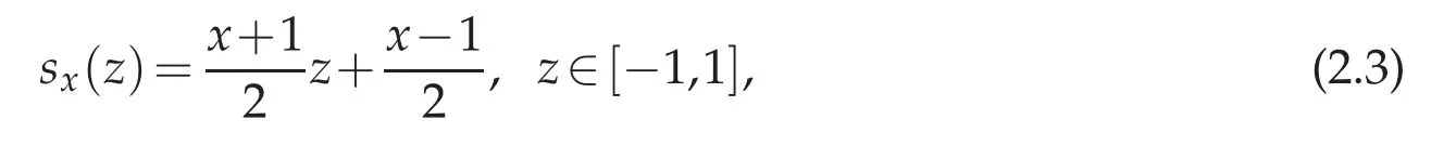
and then(2.2)becomes
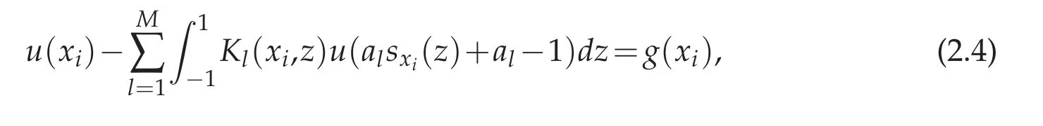
where Kl(x,z)
Next using a N+1-point Gauss quadrature formula gives
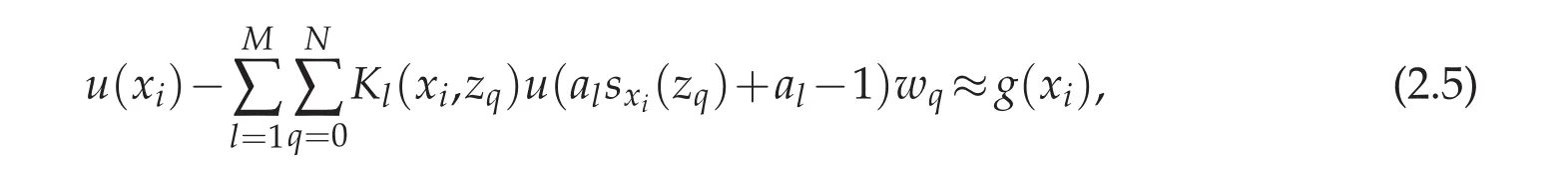
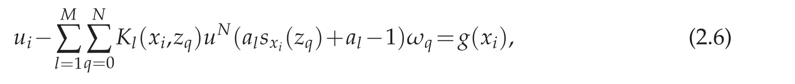
for i=0,1,...,N,where zqare the N+1 Legendre Gauss,or Legendre Gauss-Radau,or Legendre Gauss-Lobatto points,corresponding weight wq,q=0,1,...,N.We use uito approximate the function value u(xi)and use
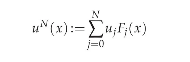
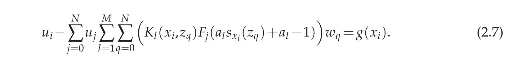
to approximate the function u(x),where Fj(x)is the j-th Lagrange basic function associated withThenthe Chebyshevspectral methodis to seek uN(x)suchthatsatisfies the following equations for i=0,1,...,N,
which is equivalent to
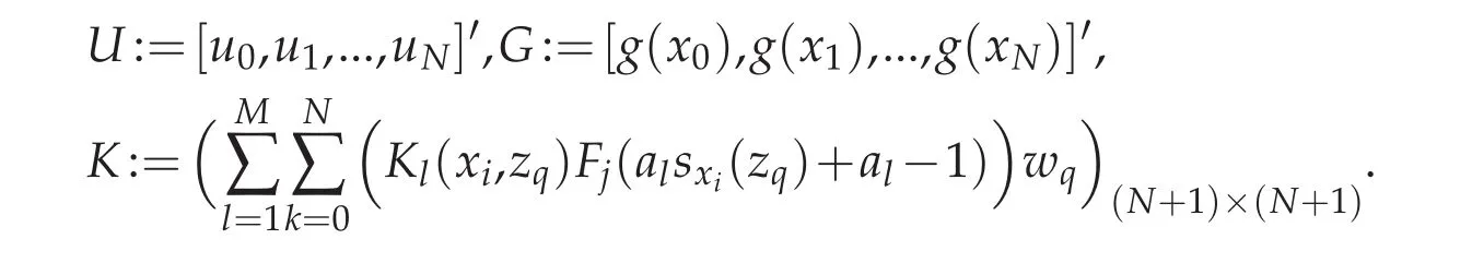
We can also write the above equation in matrix form of U?KU=G,where
3 Some spaces and lemmas
In this section we will introduce some spaces and lemmas that are prepared for the error analysis.First for non-negative integer m,we define
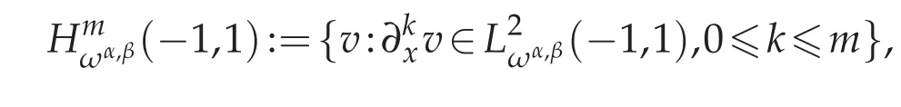
with the norm
But in bounding the approximation error,only some of the L2-norms appearing on the right-hand side of the above norm enter into play.Thus,for a nonnegative integer N,it is convenient to introduce the semi-norm
Particularly when α=β=0,we denoteWhenwe denote
And the space L∞(?1,1)is the Banach space of the measurable functions u:(?1,1)→R,which are bounded outside a set of measure zero,equipped the norm
Lemma 3.1([8,15]).Let Fj(x),j=0,1,...N are the j-th Lagrange interpolation polynomials associated with N+1 Chebyshev Gauss,or Chebyshev Gauss-Radau,or Chebyshev Gauss-Lobatto pointsThen

whereINis the interpolation operater associated with the N+1 Chebyshev Gauss,or Chebyshev Gauss-Radau,or Chebyshev Gauss-Lobatto pointspromptly
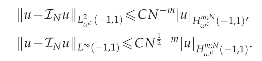
Lemma 3.2([6,17]).Assume that u∈m≥1,then the following estimates hold
Lemma 3.3([6,17]).Suppose uv∈Hm(?1,1)for some m≥1 and ψ∈PN,which denotes the space of all polynomials of degree not exceeding N.Then there exists a constant C independent of N such that
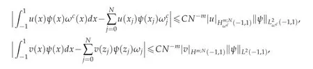
where xjis the N+1 Chebyshev Gauss,or Chebyshev Gauss-Radau,or Chebyshev Gauss-Lobatto point,corresponding weight,j=0,1,...N and zjis N+1 Legendre Gauss,or Legendre Gauss-Radau,or Legendre Gauss-Lobatto point,corresponding weight ωj,j=0,1,...N.
Lemma 3.4([12,18]).(Gronwall inequality)Assume that u(x)is a nonnegative,locally integrable function defined on[?1,1],satisfying
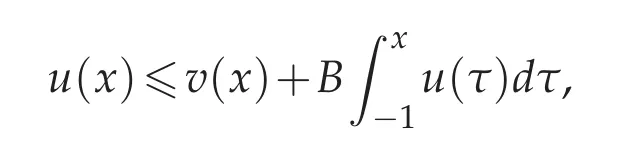
where B≥0 is a constant and v(x)is integrable function.Then there exists a constant C such that
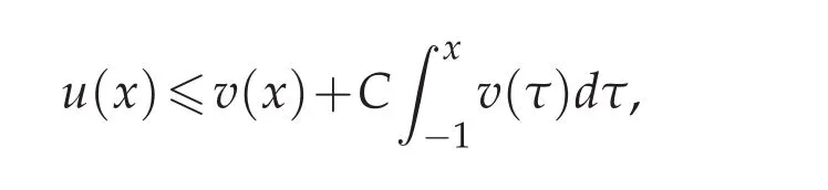
and

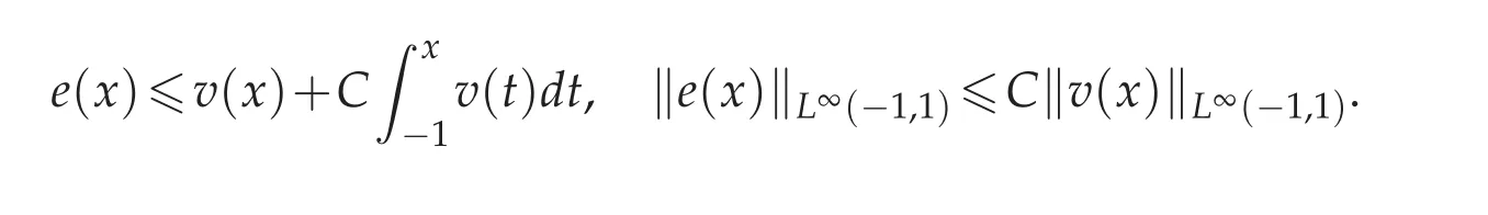
Lemma 3.5.Suppose 0≤B1,B2,...,BM<+∞.If a nonnegative integrable function e(x)satisfies
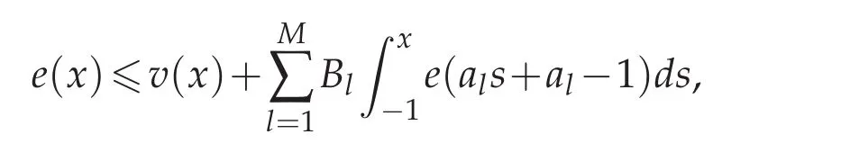
where v(x)is a nonnegative function too.Then there exists a constant C such that
Lemma3.6([13]).Forallmeasurable function f≥0,the following generalized Hardy’s inequality
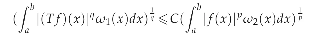
holds if and only if
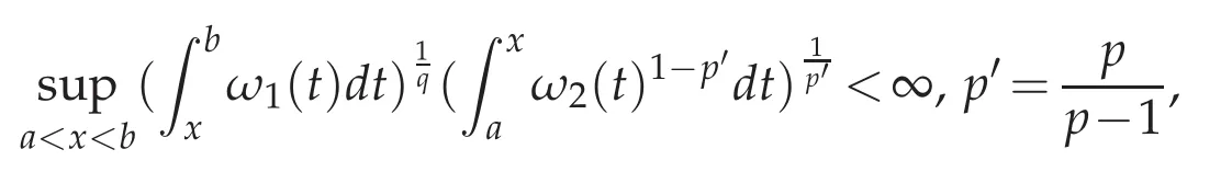
for the case 1<p≤q<∞.Here,T is an operator of the form
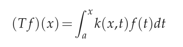
with k(x,t)a given kernel,ω1,ω2weight functions,and?∞≤a<b≤+∞.
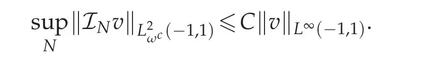
Lemma 3.7([13,16]).For all bounded function v(x),there exists a constant C independent of v such that
4 Error analysis
Now we turn to give the main result of the article.Our goal is to show the rate of convergence decay exponentially in the infinity space and the Chebyshev weighted Hilbert space.Firstly we carry out our analysis in L∞space.
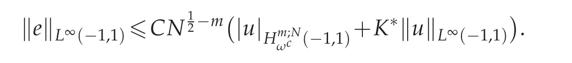
Theorem 4.1.Assume that u(x)is the exact solution of(2.1)and uN(x)is the approximate solution achieved by Chebyshev spectral method from(2.6).Then for N sufficiently large,we get

where

Proof.Make subtraction from(2.4)to(2.6)and we have
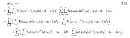
If we let e(x)=u(x)?uN(x)and(4.2)turns into
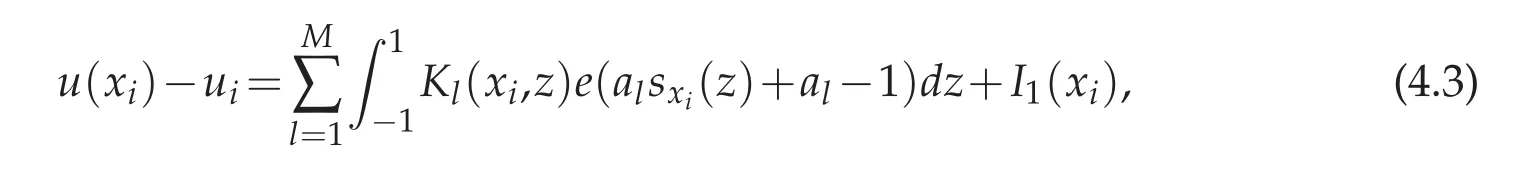
where

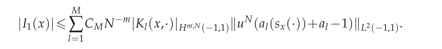
To estimate I1(x),using Lemma 3.3,we deduce that
We multiply Fi(x)on both sides of(4.3),sum up from i=0 to N and get
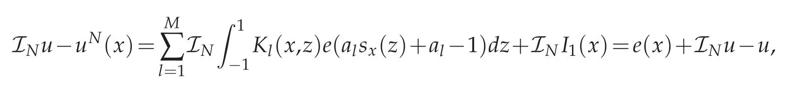
subsequently,
where

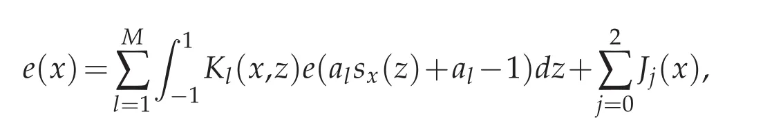
We rewrite e(x)as follows by using the inverse process of(2.3)
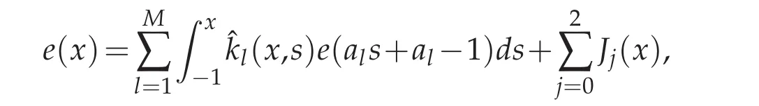
then we have
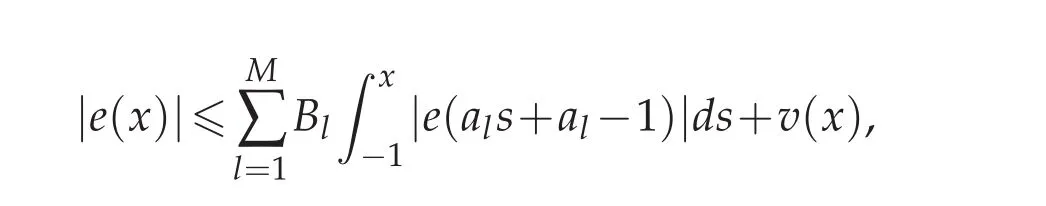
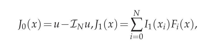
where
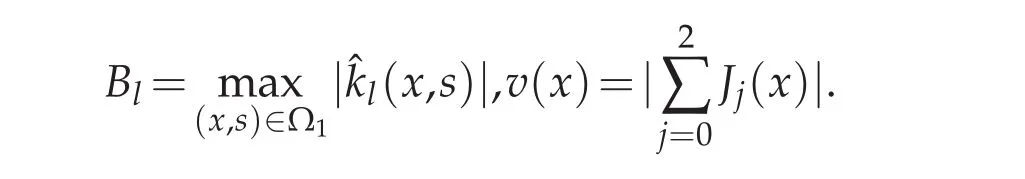
Using Lemma 3.5,we obtain
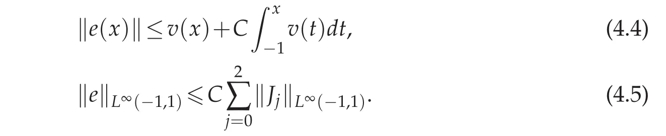
Now we come to estimate each Jj(x).First to reckon ‖J0‖L∞(?1,1),with the help of Lemma 3.2,we get

Then for the evaluate of J1(x),using Lemma 3.3,we know that

together with Lemma 3.1,we have
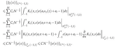
In order to bound J2(x),apply the secnod conclusion in Lemma 3.2 and let m=1 and we yield
From what has been discussed above,we yield

Since for N sufficiently large,logN<,therefore we get the desired estimate
So we finish the proof of Theorem 4.1.
Next we will give the error analysis inspace.
Theorem 4.2.Assume that u(x)is the exact solution of(2.1)and uN(x)is the approximate solution obtained by Chebyshev spectral method from(2.6).Then for N sufficiently large,we get

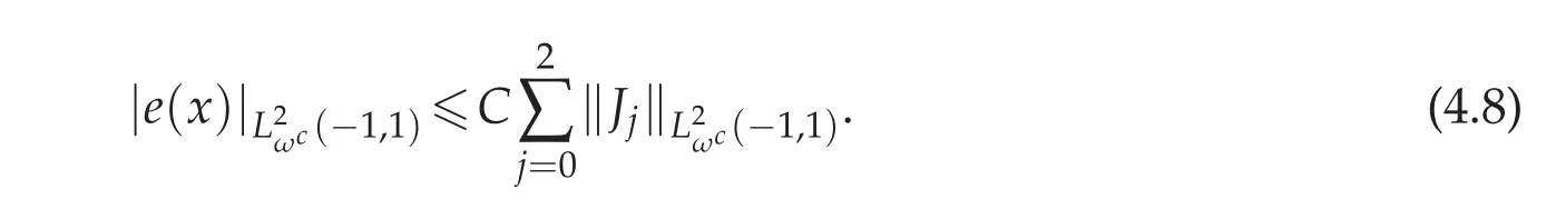
Proof.The same method followed as the first part of Theorem 4.1 to(4.4),and by Lemma 3.6,we have
Now we come to bound each term of the right-hand side of(4.8).First applying Lemma 3.2 to J0(x)gives:


Furthermore,if we let m=1 in Theorem 4.1,we have
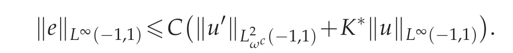
Consequently,

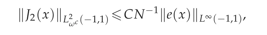
To bound ‖J2(x)‖L2ωc(?1,1),with the help from the first conclusion in Lemma 3.2,if we let m=1,as the same analysis in Theorem 4.1 for‖J2(x)‖L∞(?1,1),we can deduce that
and furthermore using the convergence result in Theorem 4.1,we obtain that

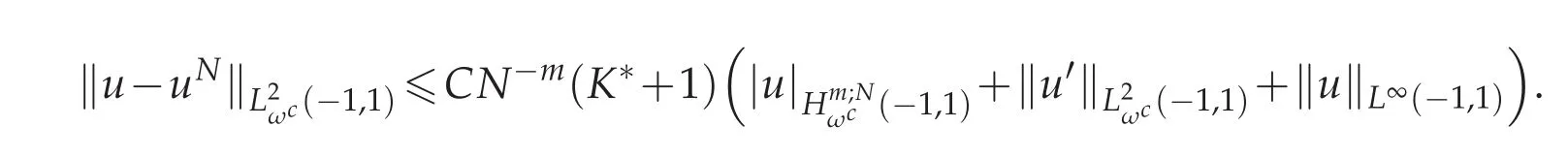
Combining(4.8)–(4.11),we get the desired conclusion
5 A numerical example
In this section,we will give numerical examples to demonstrate the theoretical result proposed in Section 4.First of all,we consider(2.1)with

The corresponding errors versus several values of N are displayed in Table 1.It is easy to find that the errors both decay in L∞andnorms.
Table 1:The errors versus the number of collocation points in L∞ andnorms.
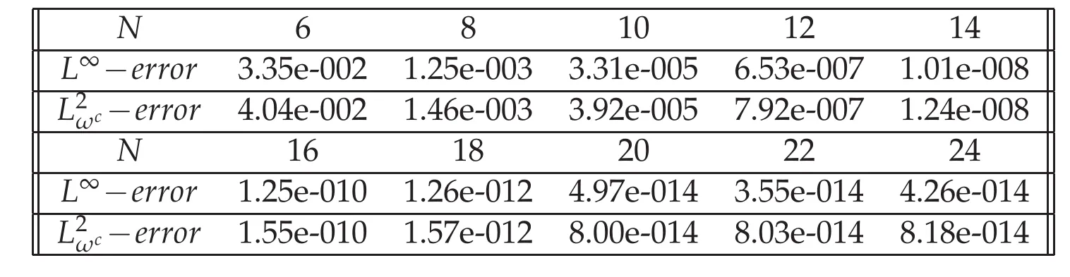
Table 1:The errors versus the number of collocation points in L∞ andnorms.
N 68 10 12 14 L∞?error 3.35e-002 1.25e-003 3.31e-005 6.53e-007 1.01e-008 L2ωc ? error 4.04e-002 1.46e-003 3.92e-005 7.92e-007 1.24e-008 N 16 18 20 22 24 L∞?error 1.25e-010 1.26e-012 4.97e-014 3.55e-014 4.26e-014 L2ωc ? error 1.55e-010 1.57e-012 8.00e-014 8.03e-014 8.18e-014
Moreover we give two graphs below.The left graph plots the errors for 6≤N≤24 in both L∞andnorms.The approximate solution(N=24)and the exact solution are displayed in the right graph.
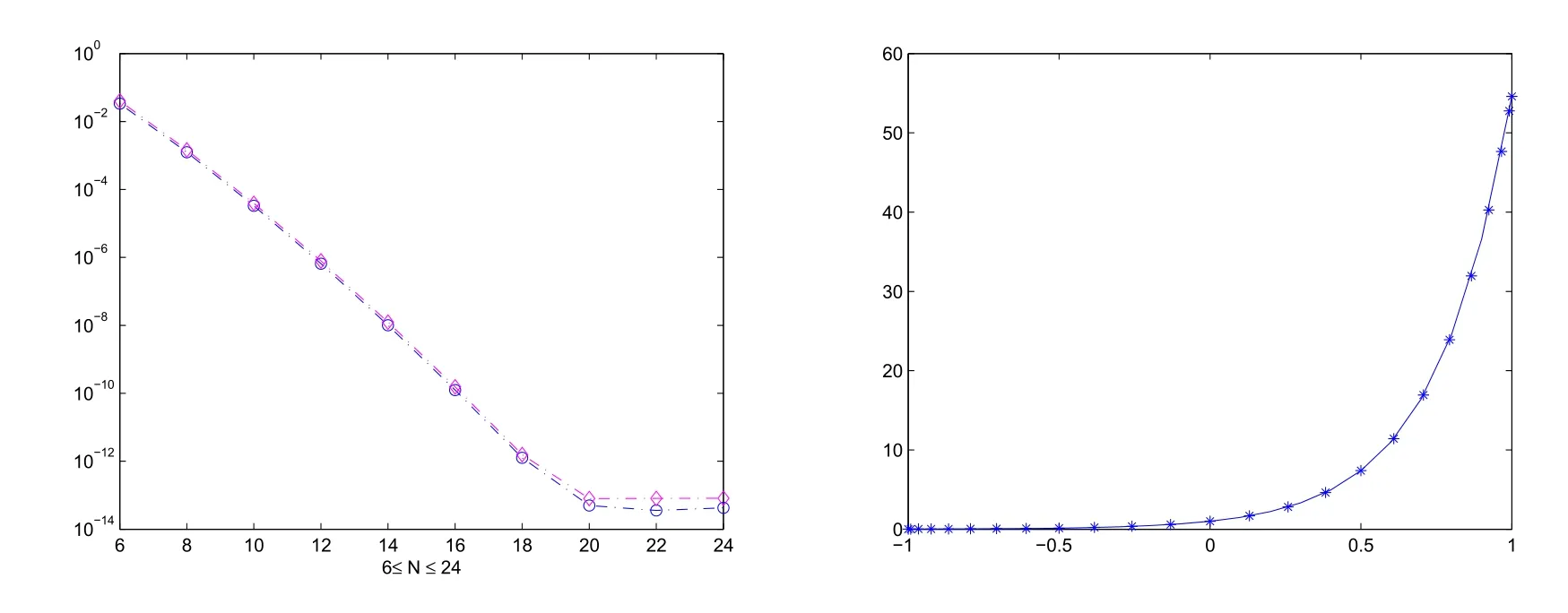
Figure 1:The errors versus the number of collocation points in L∞ andnorms(left).Comparison between approximate solution and the exact solution(right).
This example has appeared in[18].Comparing the errors in[18]and ours,one is easy to find that the accuracy obtained by Chebyshev is higher than the Legendre spectral method.Without lose of generality,we will give another example to confirm our theoretical result.
Table 2:The errors versus the number of collocation points in L∞ and norms.
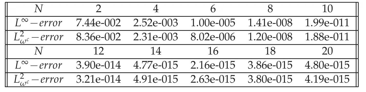
Table 2:The errors versus the number of collocation points in L∞ and norms.
N 2468 10 L∞?error 7.44e-002 2.52e-003 1.00e-005 1.41e-008 1.99e-011 L2ωc ? error 8.36e-002 2.31e-003 8.02e-006 1.20e-008 1.88e-011 N 12 14 16 18 20 L∞?error 3.90e-014 4.77e-015 2.16e-015 3.86e-015 4.80e-015 L2ωc ? error 3.21e-014 4.91e-015 2.63e-015 3.80e-015 4.19e-015
Nowwe consider(1.1)with T=2,M=2,?(t+ξ),and
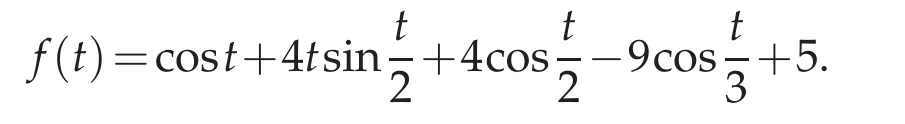
The exact solution is y(t)=cost.
There are also two graphs below.In the same way,the errors for 2≤N≤20 in both L∞andnorms are displayed in the left graph.The numerical(N=20)and the exact solution are displayed in the right graph.Moreover,the corresponding errors with several values of N are displayed in Table 2.As expected,the errors decay exponentially which are found in excellent agreement.
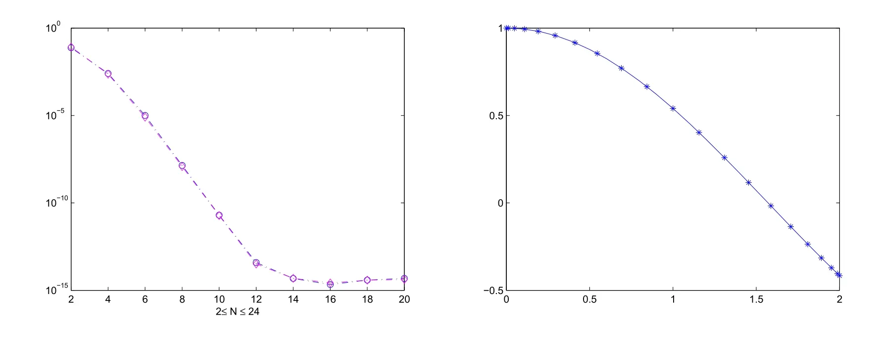
Figure 2:The errors versus the number of collocation points in L∞andnorms(left).Comparison between approximate solution and the exact solution(right).
6 Conclusion
In this paper,we successfully provide a rigorous error analysis for the Volterra integral equation with multiple delays by Chebyshev spectral method.We get the conclusion that the numerical error both decay exponentially in L∞andnorms.Moreover the accuracy obtained by our paper is higher than the Legendre spectral method.
Acknowledgments
This work was supportedby NSF of China No.11671157,No.91430104 and No.11626074 and Hanshan Normal Uninversity project No.201404 and No.Z16027.
 Journal of Mathematical Study2018年2期
- Journal of Mathematical Study的其它文章
- Ill-posedness of Inverse Diffusion Problems by Jacobi’s Theta Transform
- Highly Efficient and Accurate Spectral Approximation of the Angular Mathieu Equation for any Parameter Values q
- POD Applied to Numerical Study of Unsteady Flow Inside Lid-driven Cavity
- Generalized Hermite Spectral Method for Nonlinear Fokker-Planck Equations on the Whole Line
- A Diagonalized Legendre Rational Spectral Method for Problems on the Whole Line