
Lattice Boltzmann model for interface capturing of multiphase flows based on Allen-Cahn equation
2022-02-24 08:58HeWang王賀FangBaoTian田方寶andXiangDongLiu劉向東
Chinese Physics B 2022年2期
關鍵詞:向東
He Wang(王賀) Fang-Bao Tian(田方寶) and Xiang-Dong Liu(劉向東)
1Key Laboratory of Energy Thermal Conversion and Control of Ministry of Education,School of Energy and Environment,Southeast University,Nanjing 210096,China2School of Engineering and Information Technology,University of New South Wales,Canberra,ACT 2600,Australia3College of Electrical,Energy and Power Engineering,Yangzhou University,Yangzhou 225127,China
A phase-field-based lattice Boltzmann model is proposed for the interface capturing of multi-phase flows based on the conservative Allen–Cahn equation(ACE).By adopting the improved form of a relaxation matrix and an equilibrium distribution function,the time derivative ?t(φu)induced by recovering the diffusion term in ACE is eliminated. The conducted Chapman–Enskog analysis demonstrates that the correct conservative ACE is recovered. Four benchmark cases including Zalesak’s disk rotation,vortex droplet,droplet impact on thin film,and Rayleigh–Taylor instability are investigated to validate the proposed model. The numerical results indicate that the proposed model can accurately describe the complex interface deformation.
Keywords: lattice Boltzmann method,phase field,multiphase flow
1. Introduction
In recent years, the research of multiphase flow has attracted significant attention in a variety of fields, such as energy, aerospace, environmental protection, life science, and beyond.[1–3]Several numerical approaches, such as the volume of fluid(VOF)method[4,5]and level-set method[6,7]have been developed to depict the movement and deformation of the interface involved in multiphase flows. However,the VOF method has the difficulty in accurately analyzing the surface normal,and the level-set method suffers the lack of mass conservation. It is also challenging for these models to capture the complex topological interface evolution in the multiphase flow systems with a large density and viscosity ratio.
During the last decades, the lattice Boltzmann (LB)method has been emerging as a powerful numerical tool for modelling a wide range of complex flows, such as multiphase flows,[8]fluid-structure interaction,[9,10]and phase change heat transfer.[11]Up to now, four types of LB models have been developed for multiphase flow,including the colorgradient model,[12–14]the free-energy-based model,[15–17]the pseudopotential model,[18–20]and the phase-field-based model.[21–29]Unfortunately, only limited papers claimed that their models are competent in handling multiphase dynamics with large density and viscosity contrasts.[14,15,18]Specifically,the color-gradient model and the free-energy-based model need correction terms involving density gradient, which may result in the numerical instability at large density ratio,to eliminate some non-Navier–Stokes terms,[16,30]while the pseudopotential LB method always suffers large spurious velocities higher than the order of~10?3around the interface. Unlike the other three models,an additional equation for the order parameter, which is used to denote different phases, is coupled in the phase-field-based LB model.Coupling the lattice Boltzmann equation(LBE)for the Navier–Stokes equations(NSE),this LB model has been extensively used to investigate multiphase dynamics with large density ratios.
Commonly, two types of governing equations,i.e., the Cahn–Hilliard equation (CHE) and the Allen–Cahn equation(ACE)are utilized in the phase-field-based LB model to characterize the evolution of order parameter. Heet al.[23]pioneered the work of modelling multiphase flows with the phase-field-based LB model involving CHE.Though the complex Rayleigh–Taylor instability(RTI)was successfully reproduced, only limited density ratio has been achieved in this model. Lee and Lin[24]devised a modified model after the inspiration of Heet al.,[23]in which a three-stage discretization scheme was proposed to improve the numerical stability under high density ratio.Nevertheless,it was proved that CHE cannot be correctly recovered in these two models. Zhenget al.[27,28]then rewrote the distribution function of CHE for its proper recovery. The model is much simpler but limited to the density-matched binary fluids. Recently, great efforts have been made to improve the numerical stability at large density ratios based on CHE.[21,25,29]Though correct CHE was obtained in these models and fruitful achievements are gained under their implementation,there are still some doubts whether the second-order CE analysis are sufficient to recover CHE,a fourth-order partial differential equation.[26,31]
In contrast,the ACE is much simpler and consistent with second-order accuracy of LBE.A quantitative comparison between two models for CHE and ACE was carried out by Wanget al.[32]The results indicated that the LB model based on ACE has better numerical stability and accuracy than that based on CHE although they have similar results. The first LB model based on ACE was developed by Geieret al.[22]which indicates that the recovered interfacial equation deviates from the ACE with some error terms. Subsequently,Renet al.[26]and Lianget al.[33]proposed a multiple-relaxationtime(MRT)and a single-relaxation-time(SRT)LBM respectively,in which a time derivative?t(φu)is introduced into the source term of the LBE.Consequently, the ACE is recovered accurately.
Owing to the proven better numerical stability of LBE with the multiple-relaxation-time (MRT) collision operator,[18,34–36]an MRT model for solving ACE is proposed in this paper. An improved form of relaxation matrix and an equilibrium distribution function are devised to eliminate the time derivative?t(φu)in this model,and the second-order CE analysis demonstrates that the correct ACE can be recovered,once an appropriate source term is chosen.Four typical benchmark cases are investigated,and the results are compared with those from the previous models to demonstrate the competence of the improved model. Note that the involved Navier–Stokes equation(NSE)is recovered by the LB hydrodynamic equation proposed by Lianget al.[33]
1.1. LB model for ACE
In the phase-field theory, the ACE in the form of convection–diffusion equation, which describes the evolution of the order parameterφ,can be written as[37]
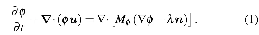
In the ACE,Mφis the mobility,andn=?φ/|?φ|is the normal vector of the interface. The order parameterφis used to identify the two-phase region,whereφl=1 andφg=0 represent the liquid phase and the gas phase,respectively. It varies smoothly across the diffused interface of the two-phase region,and usually the order parameter ofφ=(φl+φg)/2=0.5 is used to characterize the gas-liquid interface. For the system with interface thicknessW,the parameterλ=?4(φ ?φl)(φ ?φg)/W.
The evolution equation of the LB model includes two steps of collision and streaming. The collision step with the multi-relaxation-time operator has the following form of
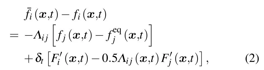
where,fi(x,t)andare the distribution functions in the velocity space before and after the collision at timeton positionx, respectively,Λis the collision matrix, andF′is the source term in the velocity space. By the left multiplication of transformation matrixM, we can transform Eq. (2) from velocity space to moment space as
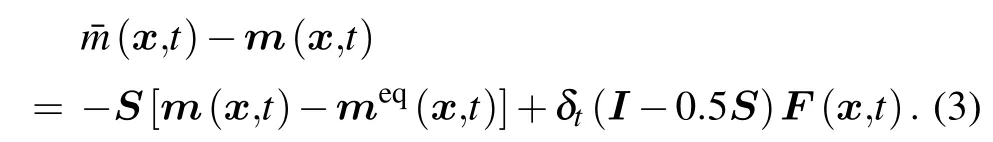
wherem(x,t)=M f(x,t) and ˉm(x,t)=are the distribution functions in the moment space before and after the collision at timetat positionx,respectively.S=MΛM?1is the relaxation matrix, andF=MF′is the source term in the moment space. For D2Q9 discrete velocity sets,the commonly used transformation matrixMis shown below:

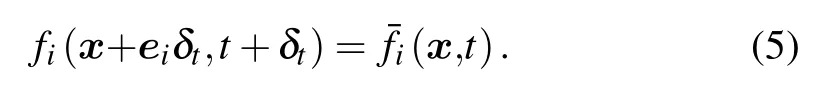
Then,the distribution function is transformed into the velocity space byM1to execute the streaming step
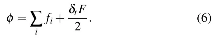
By taking the first-order moment offi,the order parameter is obtained as follows:
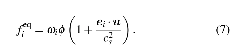
To correctly recover ACE,it is necessary to select a desirable relaxation matrix and an equilibrium distribution function.From the view of the advection–diffusion equation,Huang and Wu[38]pointed out that for D2Q9 once the relaxation matrix is diagonal,and the equilibrium distribution function is designed as
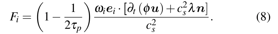
An error term related to?t(φu) will be inevitably generated when the advection–diffusion equation is recovered into the ACE. They found that the error term originates from the disturbance caused by the recovered convection term on the firstorder scale to the recovered diffusion term on the second-order scale, which cannot be eliminated simply by designing the equilibrium distribution function. To completely eliminate the effect of the error term on multiphase flow simulations,Lianget al.[33]proposed that the time derivative term?t(φu)should be introduced into the source term
A similar work was done by Renet al.[26]However,the term?t(φu) was discretized by an explicit Euler scheme for simplicity in their work.
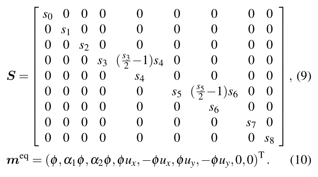
For the purposes of recovering the accurate ACE and avoiding the possible numerical errors,we further improve the work of Huang and Wu,[38]in which a new form of relaxation matrix and an appropriate equilibrium distribution function are designed as shown in Eqs.(9)and(10),respectively
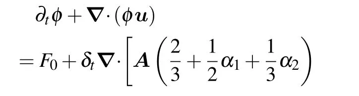
A Chapman–Enskog analysis(see Appendix A)demonstrates that the ACE can be correctly recovered with Eqs.(9)and(10).Settings3=s5, we can finally obtain the following macroscopic equation:

By comparing Eq.(11)with the ACE in Eq.(1),some parameters can be figured out as
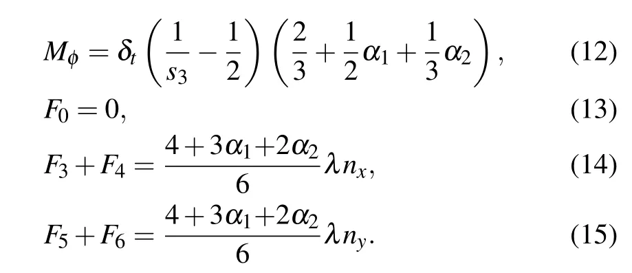
Here, the parameters take the following values:α1=?2,α2=2, andF4=F6=0. Then equation (11) is simplified and the resulting equation is just the same as ACE.That is to say,the ACE is recovered correctly without any error terms by using the modified relaxation matrix and source term.
2. Numerical results
In this section,four benchmark cases,including Zalesak’s disk rotation, vortex droplet, droplet impact on thin film, and Rayleigh–Taylor instability,are investigated to validate the interface capture capability of the improved model. The LB model for incompressible NSE in Ref.[33]is utilized to characterize the multiphase fluid flows involved in the latter two cases. In Ref.[33],the following governing equations for incompressible fluid flow are recovered:
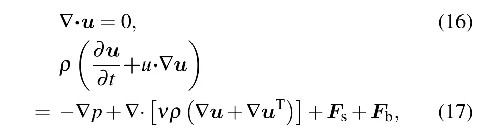
whereρis the density of the fluid,uis the velocity,pis the pressure,νis the kinematic viscosity,Fs=μ?φis the surface tension force,andFbis the body force.The chemical potentialμis given as follows:
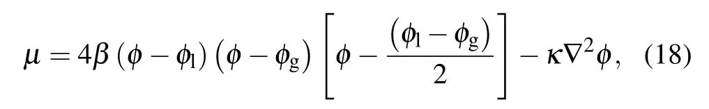
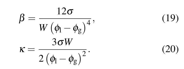
where the parametersβandκare both a function of interface widthWand surface tension coefficientσ, and given as follows:
It is noted that the interface thicknessWis set to be 2 in lattice units in the test of Zalesak’s disk rotation and vortex droplet, andW= 5 is chosen in the other two cases. For numerical stability, the order parameter should be initialized smoothly across the interface.The hyperbolic tangent function is adopted to form a two-phase diffuse interface.[25]Our improved model(denoted as MRT2)is compared with two models: the SRT model by Lianget al.[33](denoted as SRT) and the MRT model by Renet al.[26](denoted as MRT1), both of which adopt an explicit Euler scheme to discretize the term?t(φu)in the source term.All the results come from the codes programed by us.
2.1. Zalesak’s disk rotation
Zalesak’s disk rotation is a classic benchmark to examine the ability of the algorithm to capture the interface. Initially,a disk with a slot is placed in the center of the periodic square computation domain with a size ofNx=Ny=L=200. The radius of the disk and the width of the slot are set to be 80 and 16 in lattice units,respectively.The disk is driven by a rotation flow field,followingu=?ω(y?0.5Ny)andv=ω(x?0.5Nx),whereω=πU0/Lis the rotating angular velocity,and the corresponding periodT=2L/U0. After one period,the interface should return to its original position. To quantitatively show the difference between two states before and after rotation,the relative error is defined as
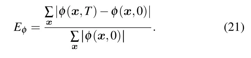
Note that the mobilityMφis directly related to the relaxation timeτp=1/s3,and thus it shows a significant influence on the numerical stability of this model. To simplify the description,the Peclet number(Pe),defined asPe=U0D/Mφβ(φl?φg)2,is introduced. Several simulations are then conducted under various values ofPewithMφvarying from 0.01 to 0.0001.The interface morphologies after rotation by all models are shown in Fig.1 and the quantitative comparisons are listed in Table 1.For the case ofPe=41.67, the disk contour att=Tshow a smoother concave corner inside the slot. All models have their own best performances atPe=2083 andPe=4167. Although the contours are almost indistinguishable, the relative error listed in Table 1 indicates that the MRT model has better accuracy in most of cases. Moreover, onceMφdecreases to 0.0001,i.e.,Pe=2083 and 4167, the MRT2 model gives a largerEφthan the other cases while the SRT model and the MRT1 model become unstable and fail in simulation. In general,the proposed MRT model shows its robustness and accuracy for various values ofPe.
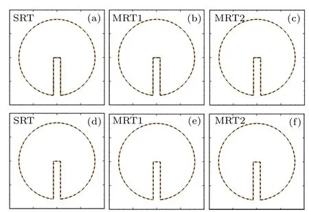
Fig. 1. Phase field contours of Zalesak’s disk rotation problem (φ =0.5,results of t =0 and t =T are plotted in black solid line and yellow dashed line)for Pe=41.67((a)–(c))and for Pe=416.7((e)–(f)).
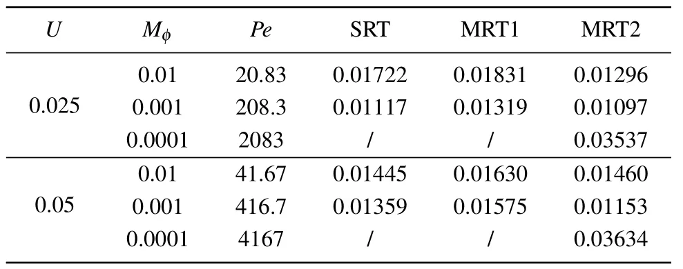
Table 1. Relative errors of Zalesak’s disk rotation.
2.2. Vortex droplet
Another benchmark of vortex droplet is investigated to further test the capability of the proposed model in capturing interface deformation. Initially, a round droplet with a radius ofR=40 is located at(100,150)in a periodic square computation domain with a size ofNx=Ny=L=200.The droplet is driven by a strongly nonlinear flow field which conforms with the following equations:
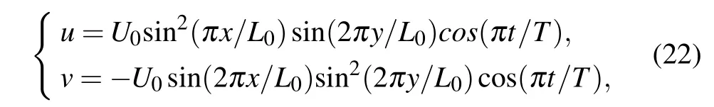
where the periodT=3L/U. Theoretically, for this velocity field, the droplet interface will undergo a severely deformed and stretched process, and return to its original position after a period. The overall topological changes of the interface solved by the proposed model atU0=0.02 andMφ=0.001 are shown in Fig.2,where we observe a helical thin filament att=T/2 and a perfect circle att=T.
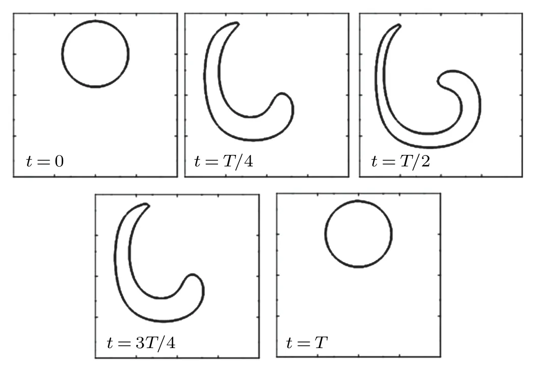
Fig.2. Interface evolutions of vortex droplet problem at different time moments(φ =0.5,results of MRT model with U0=0.02,Mφ =0.001).

Fig.3. Phase field contours of vortex droplet problem at t=T (φ =0.5,results of t=0 and t=T are plotted in black solid line and yellow dashed line),for U0 =0.02 and Mφ =0.01 ((a)–(c)), and U0 =0.004 and Mφ =0.0001((d)–(f)).
Quantitative comparisons among the three models with various values ofU0andMφare summarized in Table 2. All models illustrate the best performance atMφ=0.001 but the worst performance atMφ=0.001 orMφ=0.0001. The contours with the largest relative error of each model are compared those in Fig.3.In the case ofU0=0.02 andMφ=0.001,the SRT model and MRT1 model give the larger relative error due to the production of some unphysical disturbances near the interface. It is apparent that the contour solved by the proposed model is less disturbed and has the least error among thethree models. In the case ofU0=0.004 andMφ=0.0001,the MRT2 model gives the largest error in the three models. However, the contour still presents a perfect circle although it has a larger error. In general,the proposed MRT model has better performance. The results of Zalesak’s disk rotation and vortex droplet demonstrate that the elimination of the term?t(φu)does contribute to a better numerical stability and accuracy.
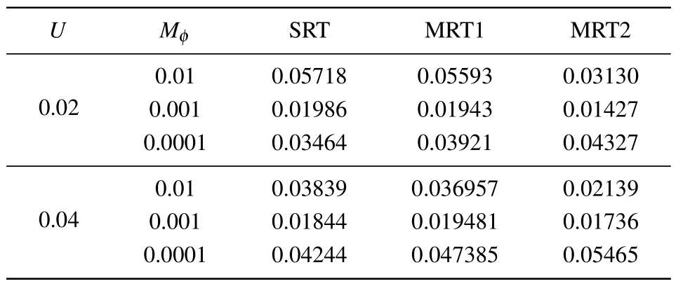
Table 2. Relative errors of vortex droplet.
2.3. Droplet impact on thin liquid film
Droplet impact on a thin liquid film widely exists in nature and engineering areas,such as the splashing of raindrops and pesticides on the plant liquid film surface,etc.[39]The reproducing of these typical free surfaces requires the higher numerical stability of the model due to the existence of a large density difference and the possible numerical singularity at the impact point. Particularly, the droplet and liquid film merging process and splashing process with possible rupture of the liquid film caused by the Rayleigh–Plateau effect desire the excellent ability of capture interface. In this subsection, the droplet impacting on the thin film with a large density ratio of 1000 is simulated based on the improved MRT-LB model.
Initially, at the bottom of the domain is spread a layer of the liquid film which a droplet is placed on, as illustrated in Fig. 4. In our simulations, the grid size is chosen to beNx=1500 andNy=500. The radius of the dropletRand the height of the liquid filmHare set to be 100 and 50, respectively. To reproduce the realistic air-water system,density values in this test are selected asρl=1000 andρg=1.0. The droplet impact velocity is(ux,uy)=(0,U)pointing to the liquid film, whereU=0.05. For simplicity, the periodic condition is imposed on the left boundary and the right boundary,and the halfway bounce-back condition is imposed on the top boundary and the bottom boundary.
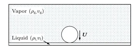
Fig.4. Schematic diagram of droplet impacting on thin liquid film.

Fig.5. Snapshots of impingement process with(a)Re=30,(b)Re=100,and(c)Re=500.
According to previous studies,[21,40,42]the dynamic behavior of droplet impinging on the liquid film can be characterized by two dimensionless parameters ofRe=2UR/νlandWe=2ρlU2R/σ. Here,simulations are carried out with a fixed Weber number ofWe=8000,and three Reynolds numbers ofRe=30,100,and 500,with the value ofνlvaried. The dynamic changes of the interface at various instants of dimensionless time scaled byt=2R/Uare shown in Fig.5. For the low Reynolds number ofRe=30, the initial kinetic energy of the droplet is absorbed by the viscous dissipation, resulting in an outward propagation of surface waves. A similar deposition phenomenon of the droplet impingement was observed experimentally by Riobooet al.[42]The effect of fluid inertia force increases with the increase ofRe, resulting in a larger interface deformation after the droplet has impacted on the film. As shown in Fig.5(b),the liquid tilts upward to form a sheet in the center and propagates to both sides. The liquid sheet tends to be like a pair of sheep horns,whose widths gradually become thinner from the head in the liquid film towards the tail in the gas. That is the ‘corona splash’ in the three-dimensional state.[42]WhenReincreases to 500,inertial forces, rather than the viscous force dominants the interfaceevolution,resulting in an obvious increase in the height of the splashing liquid sheet. The rising liquid sheet tends to bend at the edge of its tail to form a finer liquid wire. Once the interface is disturbed,the liquid wire will break into multiple droplets as shown in Fig.5(c),which is regarded as the result of the Rayleigh–Plateau effect.
The quantitative results of the spreading radius evolution along time is evaluated next.With largeReandWe,the spreading radius,r, of the coronal spray after impact usually obeys the following power-law relationship:
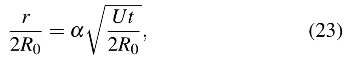
where the expansion factorαis related to the flow geometry.Josserand and Zaleski[41]fitted the relation between spreading radius and time for the three-dimensional modeling of droplet splashing,according to Eq.(23),and found thatα ≈1.1.However,the droplet is a planar disc rather than a sphere in the twodimensional simulation carried out here. Previous research has shown that the expansion factorαshould be larger than 1.1. Figure 6 shows the evolution of the spreading radius atRe=100 and 500. In a short time after the impact,the viscous effects are negligible. Hence there is no apparent dependence of the spreading radius on the Reynolds number. The numerical results under the two conditions are in overall accordance with the power law ofα=1.35.
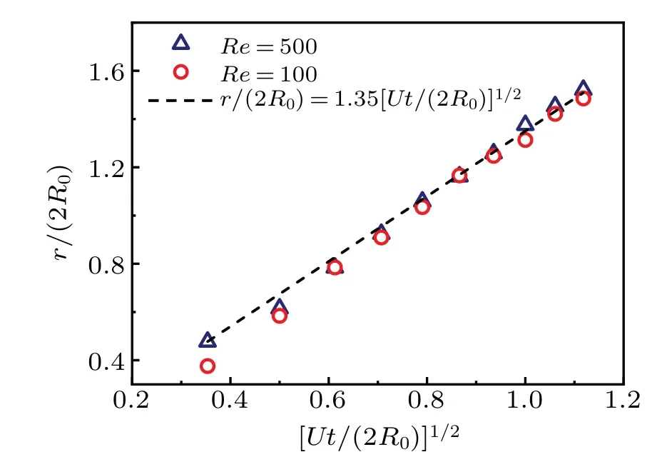
Fig.6. Evolution of spreading radius with Re=100 and Re=500.
2.4. Rayleigh-Taylor instability
Finally, a complex interface evolution induced in Rayleigh–Taylor instability (RTI) is studied to show the capacity of the present model. Here, RTI usually occurs when one layer of heavy fluid is placed on the top of another layer of lighter fluid in the downward gravity field. Any disturbance will grow to produce spikes of heavy fluid penetrating into the lighter fluid, and bubbles of light fluid moving upward. Because of its significant role in engineering applications, such as inertial confinement fusion and meteorology, RTI has attracted sustained attention for a long time.
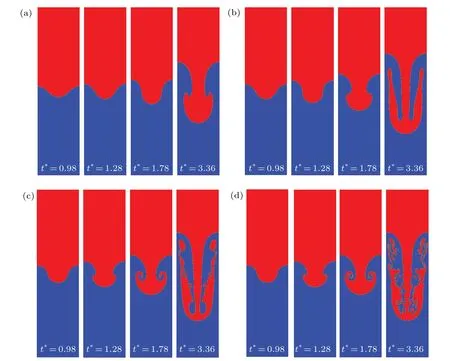
Fig.7. Interface evolution of RTI with Re=30(a),150(b),3000(c),and 30000(d).
In our simulation, the grid size of the computational domain isNy=4Nx=4Lw. The periodic boundary condition is applied to thexdirection and the halfway bounce-back boundary condition is imposed on both the top wall and the bottom wall. The fluid with densityρlandρgare arranged in the upper and lower layers respectively with an initial two-phase interface position ofh= 2Lw+0.05Lwcos(2πx/Lw). The other simulation parameters are set to beLw=256,ρl=1.0,σ=5.0×10?5. The numerical results are shown in the dimensionless form with length scalel0=Lw, and time scale, wheregis the gravity andAis the Atwood number ofA= (ρl?ρg)/(ρl+ρg). Reynolds number ofis still adopted to characterize the RTI.
First,we simulate the evolution of the RTI interface when A is small(A=0.1). Four cases of RTI underRe=30, 150,3000, and 30000 with obvious differences in interface evolution are shown in Fig. 7. Owing to the effect of gravity, the heavy fluid falls into the lighter fluid and forms a spike,while the lighter fluid surges upward to fill the gap,forming a bubble.Two typical phenomena of the roll-up of heavy fluid and the interface rupture on both sides of heavy fluid during the interface evolution of RTI are both reproduced in this simulation.According to these two phenomena, we compare the characteristics of RTI under different values ofRe. WhenRe=30,the dominant viscous effect makes the interface more stable.The spike keeps on growing downward until two sides of the spike roll up att?=3.36,and no interface rupture is observed in the simulation time. However, in the case of high values ofRe,the rolling time advances to 1.78(Re=3000)and 1.28(Re=30000), respectively. After that, the two vortices gradually grow and subsequently generate a pair of secondary vortices in the upward direction.Finally,the interface experiences a chaotic rupture,resulting in the formation of a large number of small discrete droplets in the system.
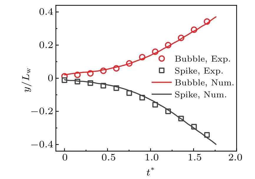
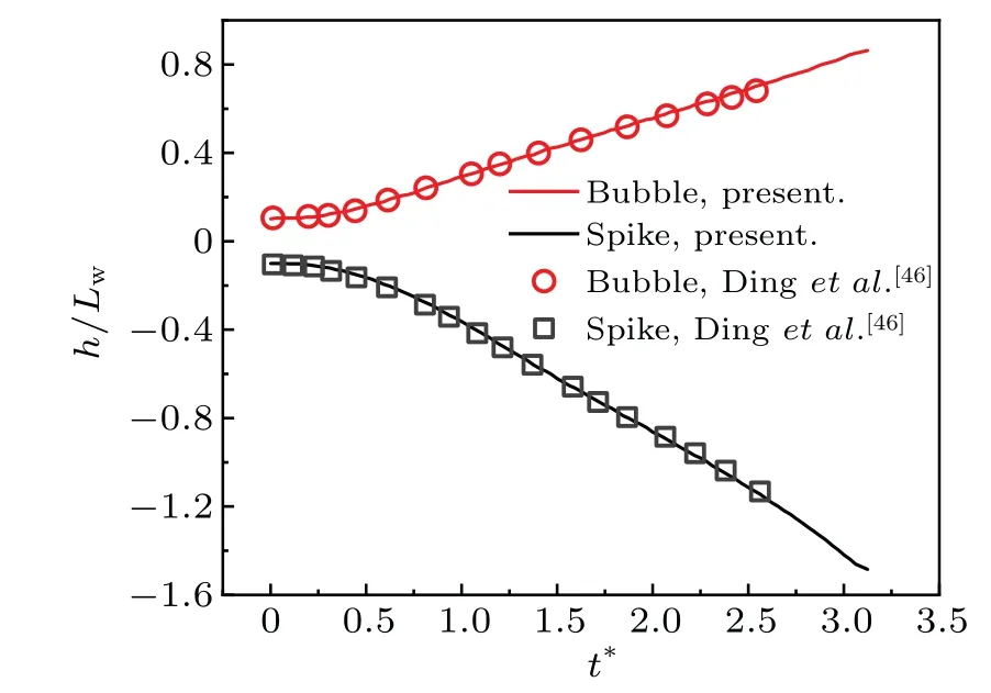
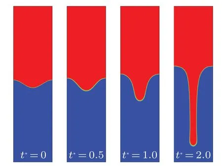
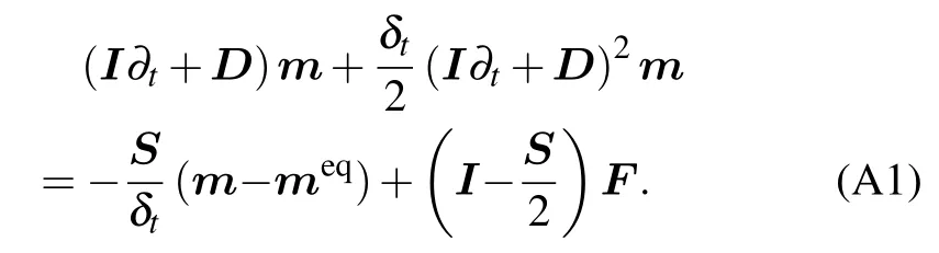
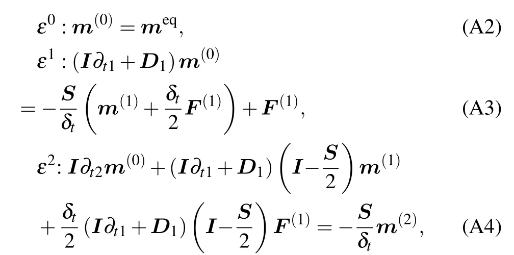
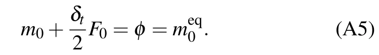
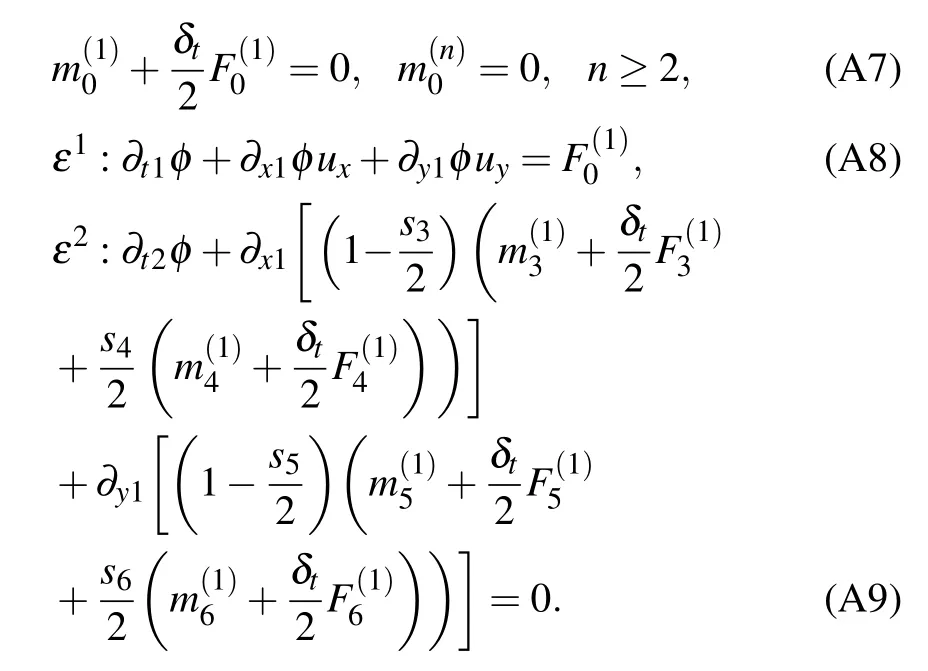
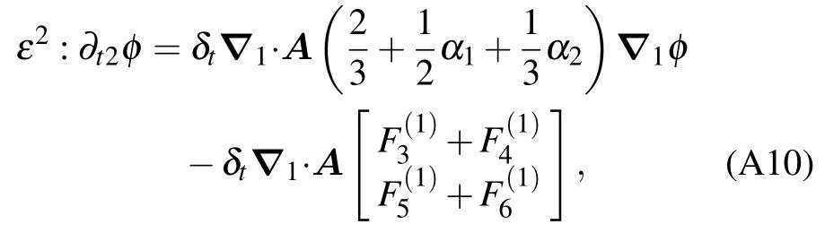
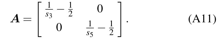
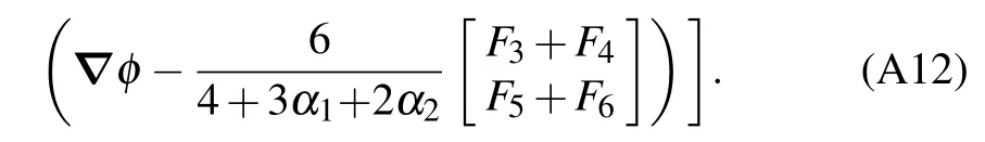
Besides, it is obvious that the viscous effect also affects the sinking velocity of the heavy fluid and the rising velocity of the lighter fluid. Figure 8 shows the time evolutions of the tip displacement and velocity of spike and bubble.The velocity is given in a dimensionless form by the Froude number ofFor the case of high value ofRe, the RTI undergoes four stages, including exponential growth, terminal velocity, reacceleration, and chaotic development.[43]In the exponential growth stage (t?≤1),the displacement of spike and bubble caused by small disturbance increase exponentially with time.[43]Then, the bubble and the spike advance at a constant speed, that is, they enter into the stage of terminal velocity (1 Fig.8. Time evolutions of displacement and velocity of bubble and spike. With time going on, the tip displacement of the bubble gradually grows to the initial disturbance wavelengthLw. At this time, the rolling up Kelvin–Helmholtz structure forming on the interface reduces the contact friction between the bubble and the spike. Besides, a momentum jet driven by the induced flow promotes the bubble to advance.[43]Therefore,the velocity in the socalled reacceleration stage(3 To further validate the present model, we carry out a simulation with similar parameters to those in the quasi-twodimensional experiment conducted by Waddellet al.[45]In their experiment, an immiscible system withA= 0.155 is driven by a body force that is 0.74 times the earth’s gravity with an initial perturbation wavelength of 54 mm. By the definition given above,we can figure out that the Reynolds number is around 5000. Figure 9 shows the time evolution of the bubble position and the spike position,obtained by the numerical simulation and cited from the experiment in Ref.[45]. It reveals that the results of the present model are in good agreement with the cited experimental results. Fig.9. Results from the present model and experimental results cited from Ref.[45]. Another case withA=0.5 andRe=3000 is alsosimulated,which is also computed by Dinget al.[46]Figure 10 provides the time evolution of the bubble position and the spike position together,and also shows the corresponding results in Ref.[46].Our results demonstrate satisfactory agreement with those cited from the literature. Fig.10. Results of the present model and cited from Ding et al.’s work.[46] Fig.11. Interface evolution of RTI with A=0.999 and Re=200. Moreover,we simulate a case withRe=200 atA=0.999,which corresponds to the density ratio of 2000. As is well known, the numerical stability is significantly restricted by the relaxation parameters. Hence, the relaxation parameters should be selected carefully to ensure a stable simulation. The interface profile att?=0,0.5,1.0,and 2.0,solved by the proposed model,presented in Fig.11,are consistent with the result in Ref. [47]. The above cases prove that the proposed model enables the interface capture of multiphase flows,with largerAapplied. However, when the Reynolds number increases to 1000,the proposed model fails to simulate the case withA=0.999. Further work needs to be done on solving the problems concurrently involving high density ratio and high-Reconditions. In this work, we propose a phase-field-based MRT LB model for interface capturing of multiphase flows based on the conservative ACE.To avoid interfering of the convection term with the diffusion term, a new form of relaxation matrix and equilibrium distribution function is adopted to eliminate the time derivative?t(φu). It is proved that the model can be recovered into conservative ACE exactly after second-order CE analysis. To validate the modified model, we first carry out a Zalesak’s disk rotation and a vortex droplet simulation to test its capability of capturing the interface. The results are compared with those from an SRT model and an MRT model, both of which adopt an explicit Euler scheme to discretize the time derivative?t(φu) in the source term. The proposed MRT model shows better numerical stability and accuracy for various mobility values among the three models.Then,the present model is tested by two transient multiphase flow problems,including droplet impact on the thin liquid film and Rayleigh–Taylor instability. Both qualitative and quantitative analyses have proved that the new model is capable of dealing with complex interface deformation. Acknowledgements Project supported by the National Key Research and Development Program of China (Grant No. 2019YFB1504301) and the Australian Research Council(Grant No.DE160101098). Appendix A:The derivation of Eq.(1) To derive the interface governing Eq. (1), we first left multiply Eq.(5)withMand substitute the result into Eq.(3)for Taylor’s expansion Here,D=M[diag(c0·?,c1·?,...,c8·?)]M?1. Then, a Chapman–Enskog(CE)analysis is carried out. Using the expansion strategies ofm=m(0)+εm(1)+ε2m(2)+···,F=εF(1),D=εD1,?t=ε?t1+ε2?t2,?=ε?1=ε(?x1,?y1)T,the consecutive orders of the parameterεcan be written as whereεis a small expansion parameter, To cancel out some terms in Eqs. (A2)–(A4), we transform Eq.(6)from velocity space into moment space and obtain Another CE expansion is conducted to obtain By substituting the equilibrium distribution function and Eq.(A6)into the conservation momentm0of Eqs.(A2)–(A4),we have The source term in Eq.(A9)can be eliminated by substituting Eq.(A3)and the equilibrium distribution function(10)into it. Thus we can obtain where the transformation matrix Here,we useds3=s5. Combining Eqs.(A8)and(A10),we can finally obtain the macroscopic Eq.(11)as follows: By comparing Eq. (A12) with the ACE in Eq. (1), some parameters in Eqs.(12)–(15)can be obtained. Takingα1=?2,α2=2,F4=F6=0,equation(A12)can be simplified just like the ACE.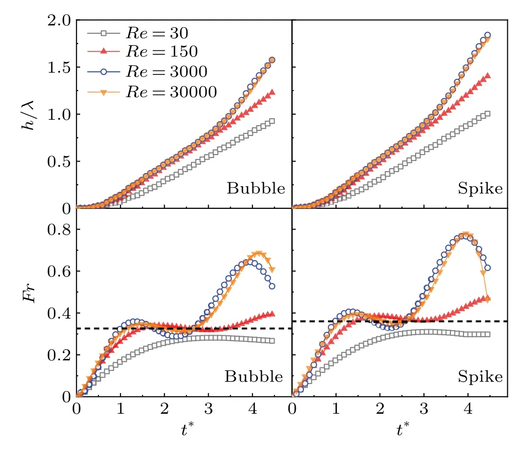
3. Conclusions


猜你喜歡
祝您健康(2022年7期)2022-07-05
河南電力(2022年3期)2022-03-18
金秋(2021年24期)2021-12-01
房地產導刊(2021年10期)2021-11-22
阿來研究(2020年1期)2020-10-28
阿來研究(2020年1期)2020-10-28
阿來研究(2020年1期)2020-10-28
藝苑(2020年1期)2020-05-06
故事大王(2019年2期)2019-03-12
初中生世界·七年級(2017年1期)2017-01-20

- Chinese Physics B的其它文章
- High sensitivity plasmonic temperature sensor based on a side-polished photonic crystal fiber
- Digital synthesis of programmable photonic integrated circuits
- Non-Rayleigh photon statistics of superbunching pseudothermal light
- Refractive index sensing of double Fano resonance excited by nano-cube array coupled with multilayer all-dielectric film
- A novel polarization converter based on the band-stop frequency selective surface
- Effects of pulse energy ratios on plasma characteristics of dual-pulse fiber-optic laser-induced breakdown spectroscopy