
CONVEXITY OF THE FREE BOUNDARY FOR AN AXISYMMETRIC INCOMPRESSIBLE IMPINGING JET*
2024-03-23 08:05王曉慧
(王曉慧)
College of Mathematics and Physics, and Geomathematics Key Laboratory of Sichuan Province,Chengdu University of Technology, Chengdu 610059, China E-mail: xiaohuiwang1@126.com
Abstract This paper is devoted to the study of the shape of the free boundary for a threedimensional axisymmetric incompressible impinging jet.To be more precise, we will show that the free boundary is convex to the fluid, provided that the uneven ground is concave to the fluid.
Key words Euler system; axisymmetric impinging jet; incompressible; free boundary; convexity
1 Introduction and Main Theorems
We consider in this paper three-dimensional inviscid, irrotational and incompressible ideal flows.In order to understand some important phenomena pertaining to ideal fluids,it is natural to start with the stationary Euler equations
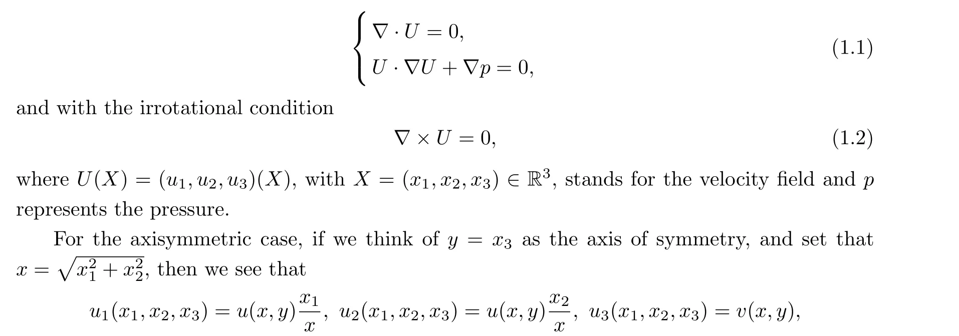
whereuandvare called the radial velocity and the vertical velocity, respectively.It is well known that,in the cylindrical coordinates,system(1.1)and the irrotational condition(1.2)can be formulated into
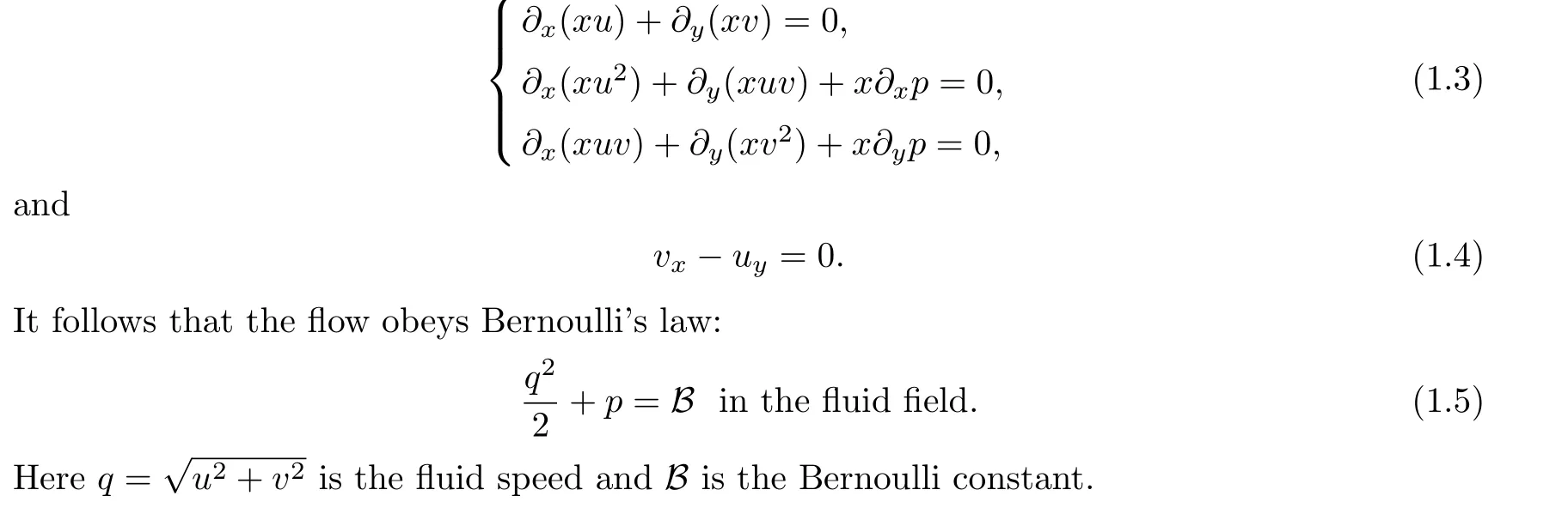
Multi-dimensional gas flows give rise to many challenging problems.Since the 1950s,tremendous progress has been made in related fields, but the steady Euler equations themselves are not easy to handle, and they also hold the free boundary.On the one hand, there has been a lot of research on nozzle flow problems(see[6,7,19,20]and the references therein).It is worth noting that the stream function formulation cannot be applied to the steady Euler equations in a three-dimensional nozzle, and that the existence theory is completely open.Therefore, the studies on the well-posedness of solutions in three-dimensional axisymmetric nozzles have also drawn much attention; the classic works here are [13-17].Transonic shock solutions to the Euler system were investigated in [18].
On the other hand, for the flow with a free boundary, Alt, Caffarelli and Friedman made a great breakthrough in the 1980s.The variational approach was put forward to prove the regularity of the free boundary in [1]; this has been a powerful tool for handling the incompressible ideal fluid with a free boundary.For example, the authors researched incompressible jet problems, with both axially symmetric flow [2] and two-dimensional asymmetric flow [3] (also in the presence of the gravity in [4]).Caffarelli and Friedman also studied the axially symmetric cavity flow in [12, 22].Recently, Cheng, Du and Xiang etc.investigated the steady incompressible plane oblique impinging jet [8], the axisymmetric impinging jet [9], R′ethy flow in the two-dimensional case [10] and the axially symmetric case [11].In this paper, as a continuation of the work of [9], we will analyse the shape of the free boundary for the axisymmetric impinging jet flow, this has important applications in aerospace, the chemical industry, environmental protection, and the petroleum and energy industries.
We define the nozzle wall as
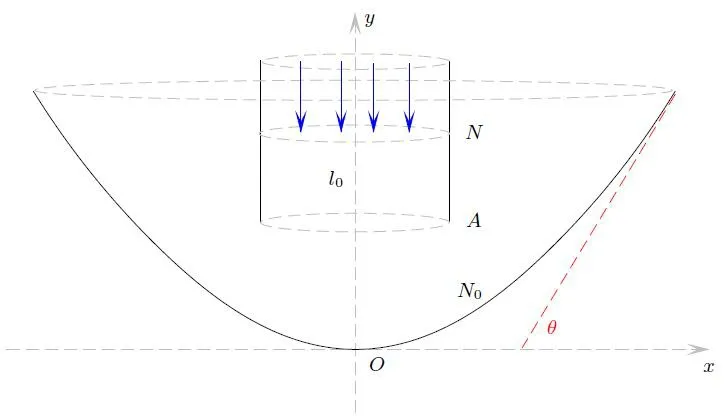
Figure 1 The semi-infinitely long nozzle and concave ground
The nozzleNand groundN0are impermeable,so that the following slip boundary condition holds:
Here→nremains the outer normal toN ∪N0.Additionally, the free boundary Γ is the surface of the material andl0is the axis of symmetry, and the condition (1.9) also holds on Γ andl0.
According to the conservation of mass equation, (1.3)1, and the boundary condition (1.9),we can assume that the incoming mass flux is a positive constantQ, namely,
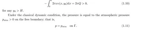
Before giving the main results of this paper,we show the well-posedness of the axisymmetric incompressible impinging jet flow, which can also be found in Theorem 2.1 in [9].
Theorem A (Theorem 2.1 in [9] - Existence of the axially symmetric incompressible impinging jet flow) Given the incoming mass flux 2πQ >0 and the atmospheric pressurepatm,if we have the nozzleNwith (1.6) and the groundN0with (1.7), then there exists a smooth solution (u,v,p,Γ) for the axisymmetric impinging jet flow satisfying that
(1) the curve Γ is expressed by a mappingy=g(x)∈C1((a,+∞)) with
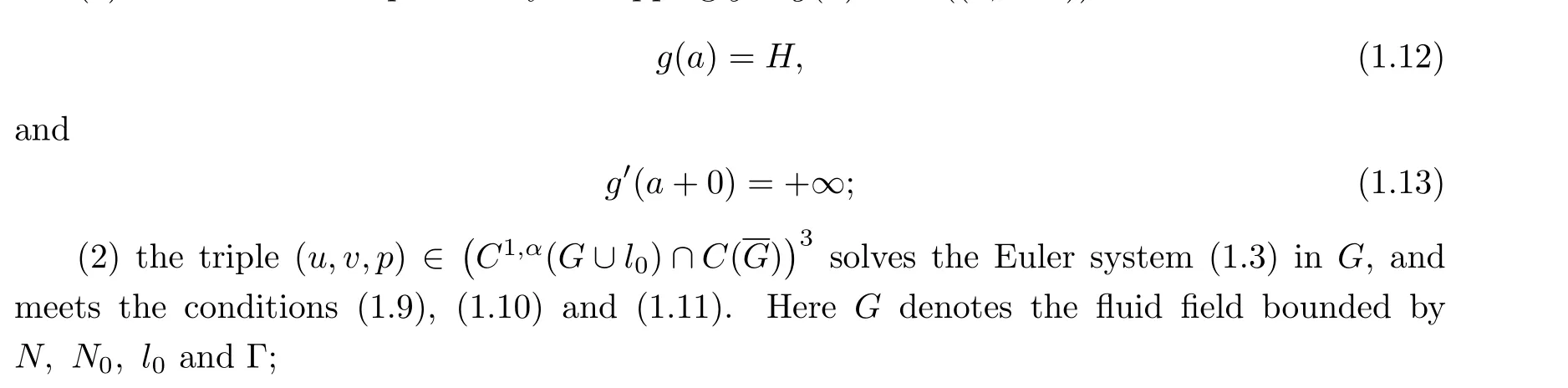
(3) the radial velocity isu >0 inG;
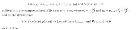
(4) the asymptotic behavior holds at the upstream
Remark 1.1The conditions (1.12) and (1.13) are the so-called continuous fit condition and the smooth fit condition, respectively.They imply that the free boundary Γ detaches smoothly from the end pointA.
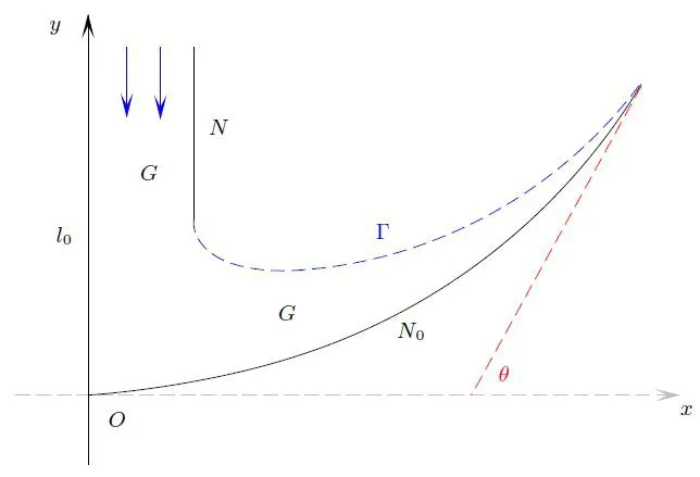
Figure 2 Convex free boundary
Next, we give our main result.
Theorem 1.2Under the hypotheses of Theorem A, if the groundN0is assumed to be concave to the fluid,that is,the functiony=K(x)satisfies the additional condition(1.8),then the free boundary Γ will be convex to the fluid (see Figure 2), namely,
Remark 1.3For the sake of clarity, we would like to point out thatN0is concave to the fluid, that is, Ω∩{y <H}and Ω∩{x >a}are convex domains.Here Ω is the possible fluid field, which is bounded byN,N0andl0.
2 The Mathematical Setting of Physical Problem
The stream function approach is a classical method for solving the three-dimensional axisymmetric flow problem.In light of the divergence free condition (1.1)1, we can introduce the stream functionψsuch that
which, together with the irrotational condition (1.4), gives thatψsatisfies the linear elliptic equation
Owing to the fact that the pressurep=patmremains constant on the free boundary Γ, it follows from Bernoulli’s law(1.5)that the fluid speedqis also a constant on Γ,which is denoted asλ, and that we can get the free boundary condition
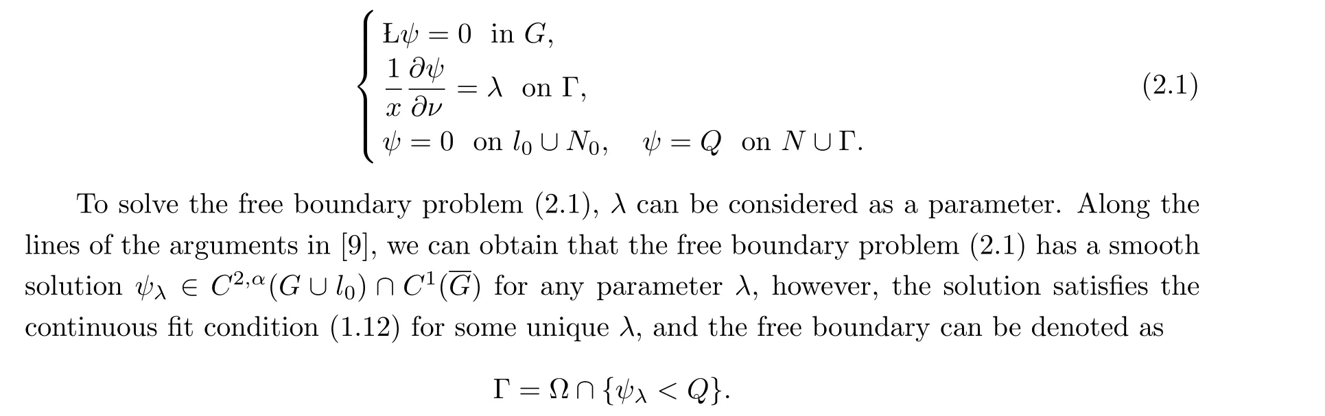
whereνis the outer normal of Γ.Therefore, the axisymmetric incompressible impinging jet problem,satisfying the conditions(1.9),(1.10)and(1.11),can be transformed into the following free boundary problem:
3 Convexity of the Free Boundary
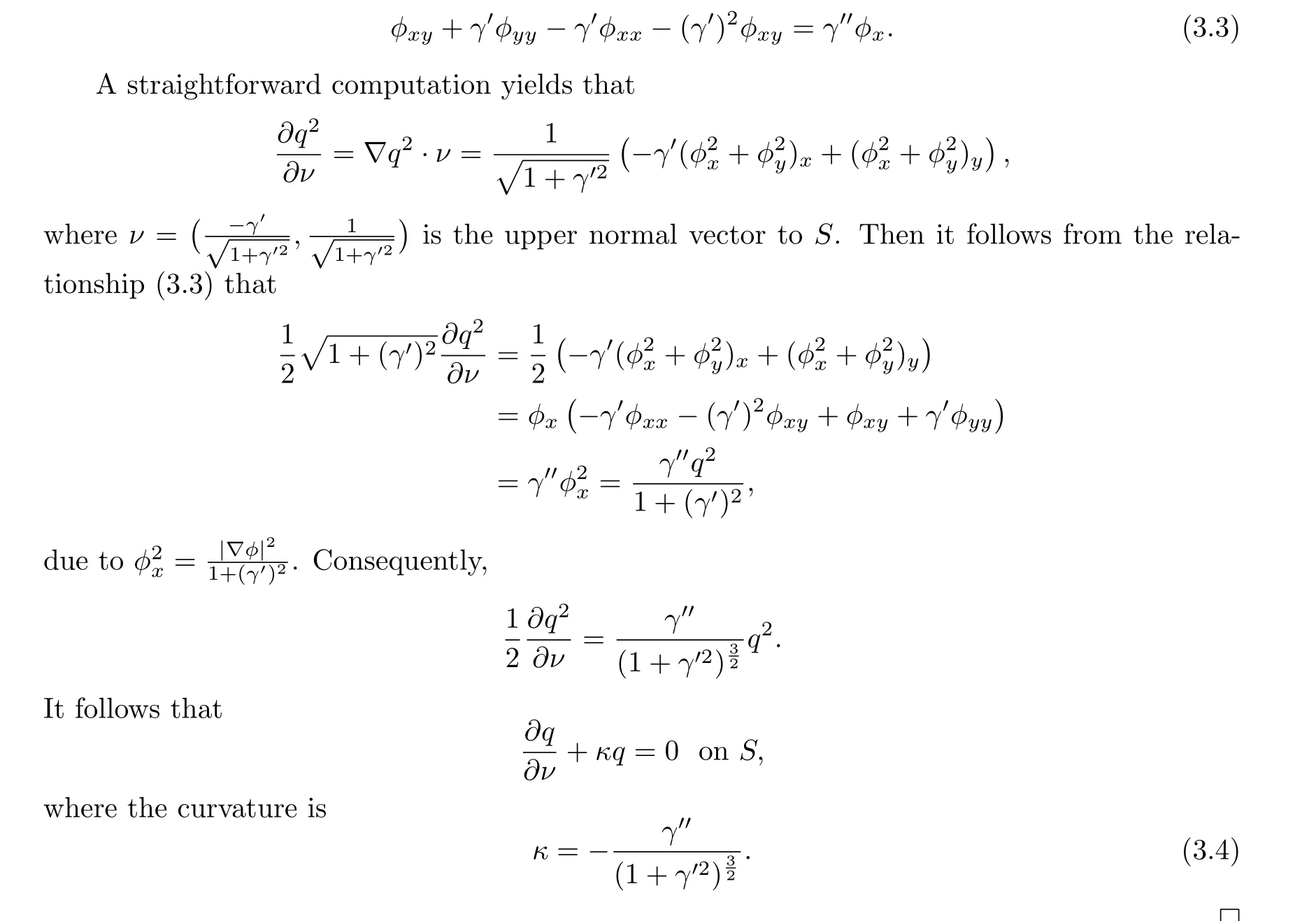
With the aid of the well-posedness of the axisymmetric impinging jet flow shown in Theorem A, we will continue, in this section, to examine the geometric shape of the free boundary.We begin by establishing the relationship between the fluid speedqand the curvatureκ.
Lemma 3.1For anyQ >0,if the streamlineS:{ψ= ~Q}with ~Q ∈[0,Q]isC2,α-smooth,then one has that
whereνis the upper normal vector to the streamlineS.
ProofThe proof of Lemma 3.1 is similar to that of the compressible case in [5].For convenience to the reader, we now give a general proof.Since the radial velocity is positive in the fluid field, namely,u >0 inG, the streamlineScan be represented by the mappingy=γ(x).Furthermore, thanks toψλ(x,y)= const.onS, it is easy to see that
Denotingφas the axially symmetric potential function of flow, it satisfies?φ= (u,v).Thus the equation (3.2) can be converted to
Therefore, taking the partial derivative of both sides of the above equation with respect tox,we can deduce that
□
We will prove that the parameterλhas a positive lower bound in the next lemma, which will be important for showing that the flow velocity attains a maximum on the free boundary.
Lemma 3.2For anyQ >0, the parameterλsatisfies that
ProofIn order to establish the inequality(3.5),we first show thatψλ(x,y)has the upper bound
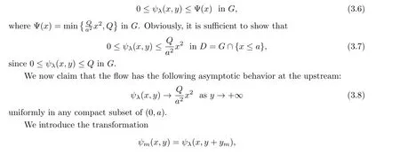
withym →+∞asm →+∞.In view of the Lipschitz continuity ofψλ(x,y), there exist a functionφ(x,y) and a subsequence, still labelled asψm, such that
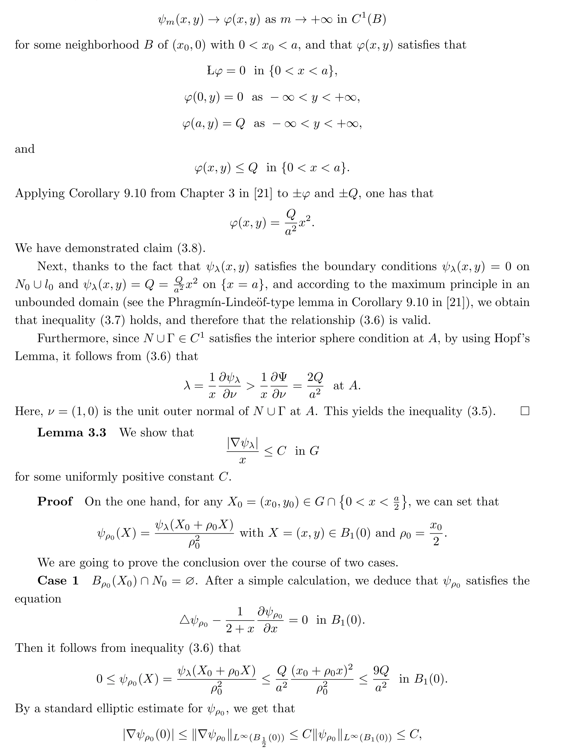
that is,
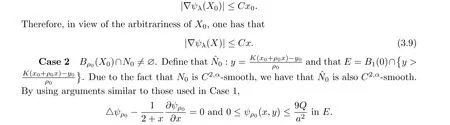
Therefore, the interior-boundary regularity of the uniformly elliptic equation yields that
Thus, (3.9) holds in this case.
On the other hand, by using the interior-boundary regularity forψλ= 0, we can obtain that the inequality (3.9) holds elsewhere inG, and therefore complete the proof.□

Lemma 3.4Under the assumptions in Theorem A, if the groundN0satisfies the additional concavity hypothesis (1.8), then the fluid speedqattains its maximum on the free boundary Γ, namely,
ProofIt is not difficult to verify thatqsatisfies that
which implies thatq2is a subsolution for a linear elliptic equation.Then, according to the maximum principle in [23], we have thatqcannot take its maximum in the interior of the fluid fieldG.Furthermore, since the flow is axially symmetric with respect tol0, we can regardl0as the interior ofG, and we also have thatqcannot get its maximum onl0.Thus,qmay attain its maximum onN ∪N0∪Γ, or at infinity.
It is easy to see that
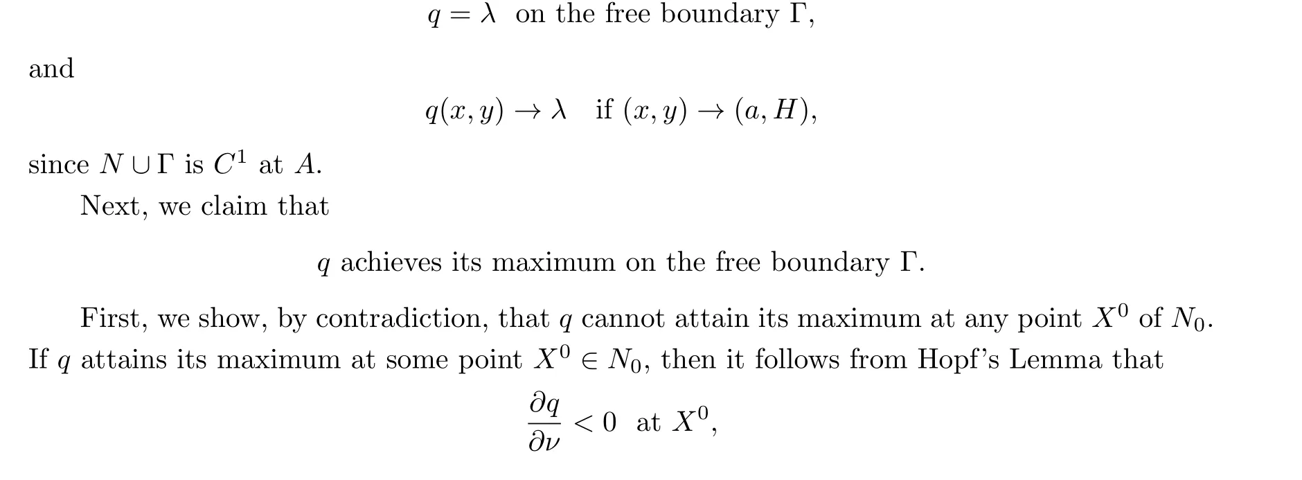
whereνis the inner vector,sinceN0∈C2,αandq ∈C1,αonN0,by elliptic boundary regularity.Consequently, it follows from (2.1) that
and then the curvature formula (3.4) yields that
This contradicts assumption (1.8).
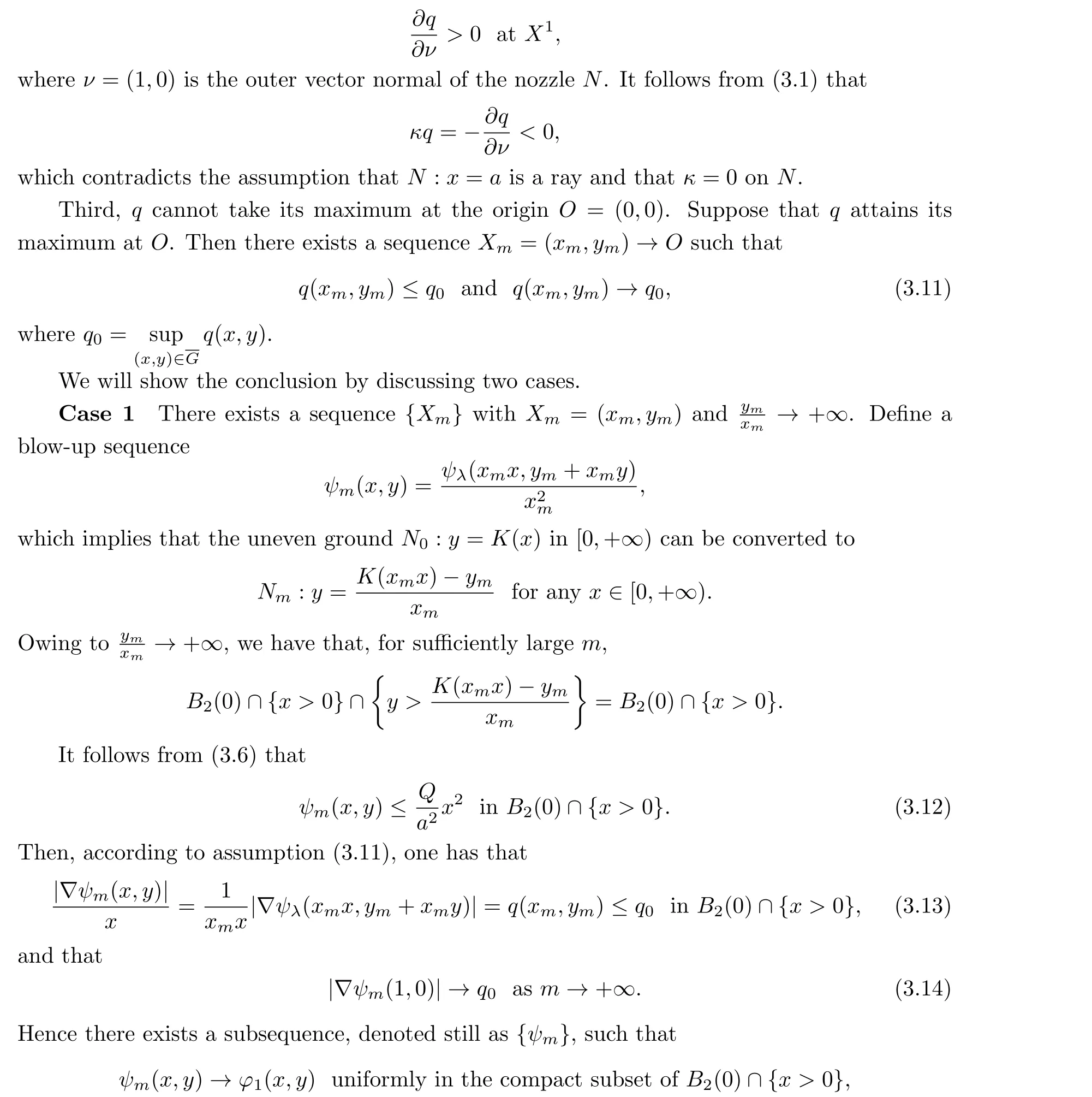
Second, we prove thatqcannot achieve its maximum at any pointX1ofN(X1/=(a,H)).Indeed, ifqachieves its maximum at some pointX1∈N, then Hopf’s Lemma yields that
and the limit functionφ1satisfies the following equation:

and the following properties hold:
which stands in contradiction to (3.5).
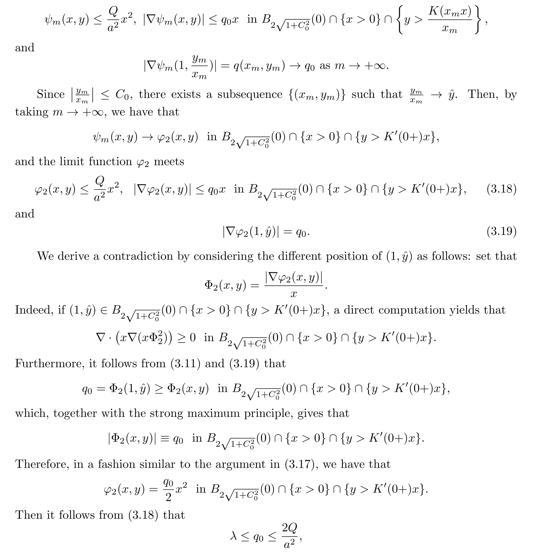
On the other hand, if we have the point (1,?y)∈l:{y=K′(0+)x}, then the maximum principle implies that
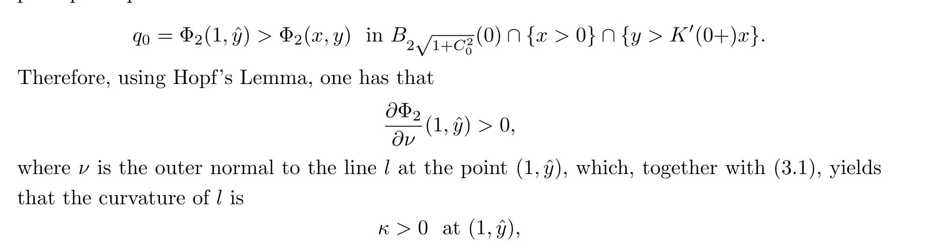
which is impossible.
Finally, suppose that we can show that
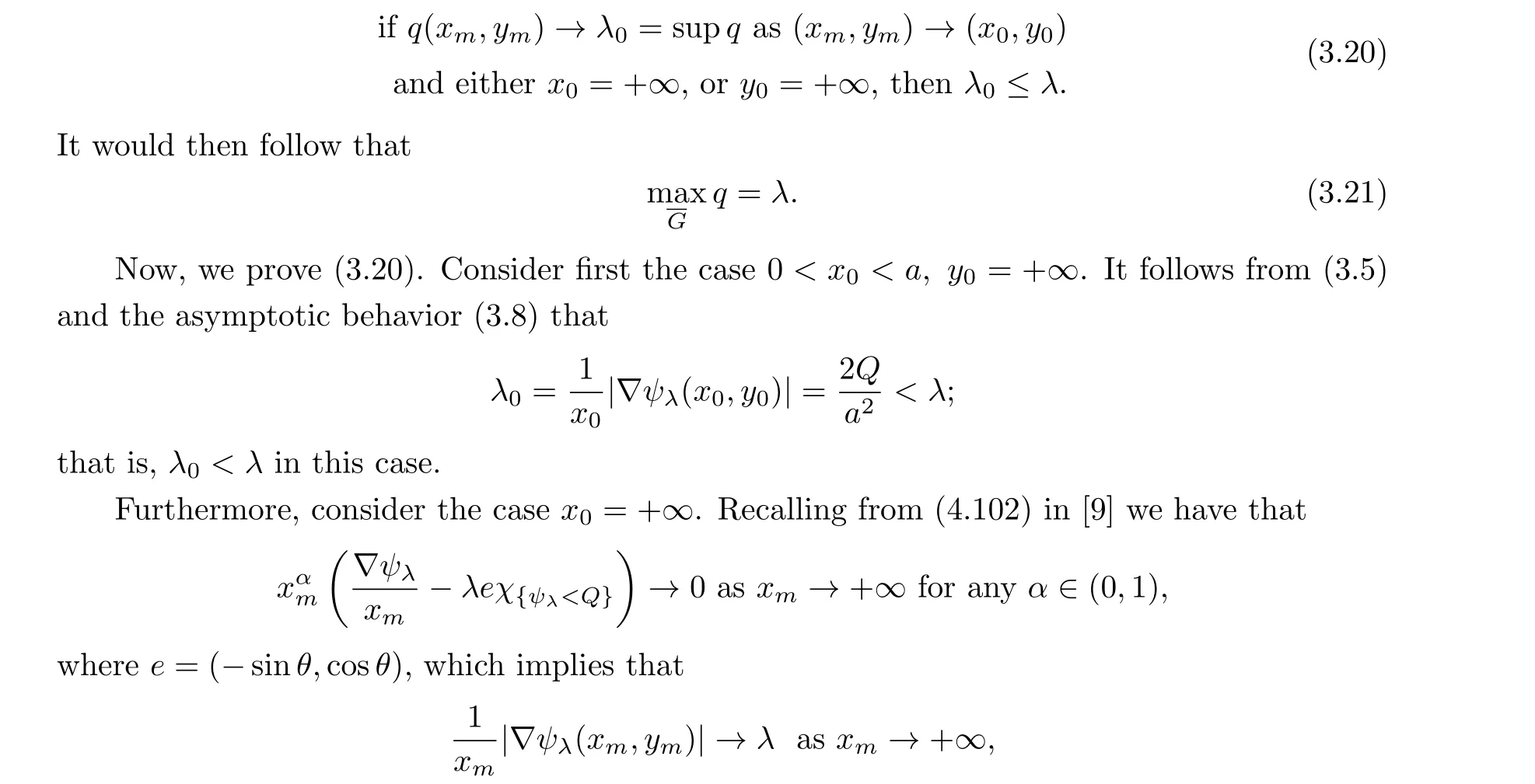
so thatλ0=λin this case.Therefore, we have proved (3.20).□
Next, with the aid of the above lemmas, we will show, in the following theorem, that the free boundary is convex to the fluid, provided that the groundN0is concave to the fluid:
Theorem 3.5Under the assumptions of Theorem A, if the groundN0also meets the condition (1.8), then the free boundary Γ is convex to the fluid, and
ProofAccording to Lemma 3.4, we obtain that the fluid speedqattains its maximum on the free boundary Γ, and therefore, it follows from Hopf’s Lemma that
whereνis the outer normal to Γ, which, together with (3.1) in Lemma 3.1, yields
that is, the curvature isκ <0 on Γ.Therefore, formula (3.4) gives thatg′′(x)>0 in (a,+∞),and we get that the free boundary Γ is convex to the fluid.□
Conflict of InterestThe author declares no conflict of interest.
 Acta Mathematica Scientia(English Series)2024年1期
- Acta Mathematica Scientia(English Series)的其它文章
- THE EXACT MEROMORPHIC SOLUTIONS OF SOME NONLINEAR DIFFERENTIAL EQUATIONS*
- GLOBAL CLASSICAL SOLUTIONS OF SEMILINEAR WAVE EQUATIONS ON R3×T WITH CUBIC NONLINEARITIES*
- SOME NEW IDENTITIES OF ROGERS-RAMANUJAN TYPE*
- NADARAYA-WATSON ESTIMATORS FOR REFLECTED STOCHASTIC PROCESSES*
- QUASIPERIODICITY OF TRANSCENDENTAL MEROMORPHIC FUNCTIONS*
- THE LOGARITHMIC SOBOLEV INEQUALITY FOR A SUBMANIFOLD IN MANIFOLDS WITH ASYMPTOTICALLY NONNEGATIVE SECTIONAL CURVATURE*