Multivariate time delay analysis based local KPCA fault prognosis approach for nonlinear processes☆

Yuan Xu,Ying Liu,Qunxiong Zhu*

College of Information Science and Technology,Beijing University of Chemical Technology,Beijing 100029,China

1.Introduction

Fault prognosis is a crucial issue to increase the reliability and safety of the industrial processes.In the literature,it has been studied with different types of approaches which can be seen from the survey papers[1–5].These approaches not only preserve robustness with changes in normal operating conditions but also prevent large deviations which would lead to a malfunction[6,7].At present,most data-driven fault prognosis methods are based on the multivariate time series.In the paper of Zhang[8],fault prognostic algorithm is developed based on multivariate relevance vector machine and time series iterative prediction.Some researchers also proposed multivariate time series prediction and statistical process monitoring methods based fault prognosis approaches[9].It can be seen that time series prediction is essential for multivariate time series based fault prognosis approach.

Time series prediction indicates the operation of forecasting a future value by analyzing the trend of past and current variable values.In this task,past and current values are acted as input while future values are generated as output[10,11].For the complex industrial process systems,the internal relationship among the process variables is complex.Mutual information is a correlation measurement method which has recently draw much attention[12,13].Multivariate correlated series could be constructed by applying mutual information to acquire the correlation among process variables.Considering back propagation(BP)network is a commonly used approach for time series prediction[14,15],the established multivariate correlated series by mutual information are taken as the inputs of BP network.In this way,the BP network could reflect the complex internal relationship and have higher prediction accuracy comparing to the original BP network.

Meanwhile,it is aware that time delay is commonly existed in the nonlinear industrial process.Traditionally,the time delay estimation always focused on computing the maximum value of the correlation or time delay mutual information between two variable's samples[16,17].A possible deflect caused by these approaches is that the transmission relationship among variables is needed as the prior knowledge.Bayesian information criterion(BIC)is an un-supervised learning algorithm which can be applied for parameter estimation through acquiring the minimum of information loss[18].For time delay estimation,it could get an optimal approximation of the time delayed series model under the information criterion.Thus the delay parameter corresponding to the minimal loss information is exactly the delay of time series.

For further fault monitoring,multivariate statistical process monitoring has been popularly applied in industrial nonlinear processes.Traditional principal component analysis(PCA)[19,20]may not be appropriate for nonlinear process due to its assumption that process variables are linear.To overcome this deficiency,kernel PCA(KPCA)[21,22]has been developed with transforming the input space to feature space.It is noted that the extracted kernel principal components may not satisfy Gaussian distribution.According to this issue,statistical local KPCA(LKPCA)[23–25]is proposed by incorporating the statistical local approach into KPCA,which overcomes the limitation of KPCA used for nonlinear process and enhances the sensitivity for incipient change detection.

This paper will introduce multivariate time delay analysis into local KPCA for incipient fault prognosis of nonlinear processes.With the introduction of mutual information estimation and Bayesian information criterion(BIC),the correlation degree and time delay of process variablesare acquired.Moreover,in order to achieve prediction,BP net work is developed for multivariate correlated time series prediction.Then LKPCA is applied to calculate two statistics to achieve fault prognosis whose input are multivariate time delayed series and future values by time series prediction.The rest of the paper is organized as follows.First,some preliminaries are given including mutual information estimation and LKPCA approach.The next section describes the way of incorporating multivariate time delay analysis into local KPCA.In Section 4,a simple nonlinear process and the Tennessee Eastman(TE)benchmark process simulation studies are given.Finally,some conclusions are made in Section 5.

2.Preliminaries

2.1.Mutual information estimation

Mutual information(MI)is a commonly used calculating correlation degree tool and sensitive to any relationship.Entropy is a fundamental prior knowledge to understand the meaning of MI.For a discrete variable x,the entropy is defined as

where piis the probability that variable x is in state i,and nxis the number of states that variable x can assume.

The joint entropy of two discrete variables,x and y,is defined as

where pijis the joint probability that variable x is in state i and variable yis in state j,nxand nyare separately the number of states that variable x and variable y can assume.

A relation between mutual information and entropy can be drawn from the above definitions.

I(x;y)is exactly the mutual information of variable x and variable y.The crucial problem of this method is the complexity of probability estimation for the variables.To avoid this,k-nearest neighbor distances method[26,27]is utilized to estimate mutual information.Its main idea is as follows: firstly define a set of n bivariate variables zi=(xi,yi),i=1,…,n and calculate the distance between sample ziand other samples.Secondly,definethe distance from zito its kth(1≤k≤n)neighbor.Thirdly,define nx(i)as the number of points xjthe distance between which and point xiis strictly less thanThe similar definition can be applied for ny(i).For the tuning parameter k,if the value is too small,the change of k will result in tremendous changes in number nx(i)and ny(i).In contrast,if the value of k is too large,the number nx(i)and ny(i)will change barely.Finally,the mutual information of two discrete variables,x and y,can be transformed as follows.

where E is the expectation operator,E[·]denotes the average value obtained from the given samples and ψ(·)is a Digamma function which can be got in iteration.

2.2.LKPCA approach

LKPCA is a new method for process monitoring which incorporates the statistical local approach into KPCA[23].This new method has been exemplified the sensitivity for incipient change detection.Suppose the original training dataset is x1,x2,… ,xn∈Rm,where m is the number of process variables and n is the sample number.Similar to KPCA,the first task of LKPCA is to get the score vector.

where tk,jdenotes the jth observation of the kth score vector,vkis the kth eigenvector of covariance matrix and ?(·)is a nonlinear mapping function to the feature space.is the coefficient indicating that the kth kernel eigenvector is spanned by observation samples in feature space.k inis a superscript.K is the centered kernel matrix.The kth eigenvector vksatisfies the following equation:

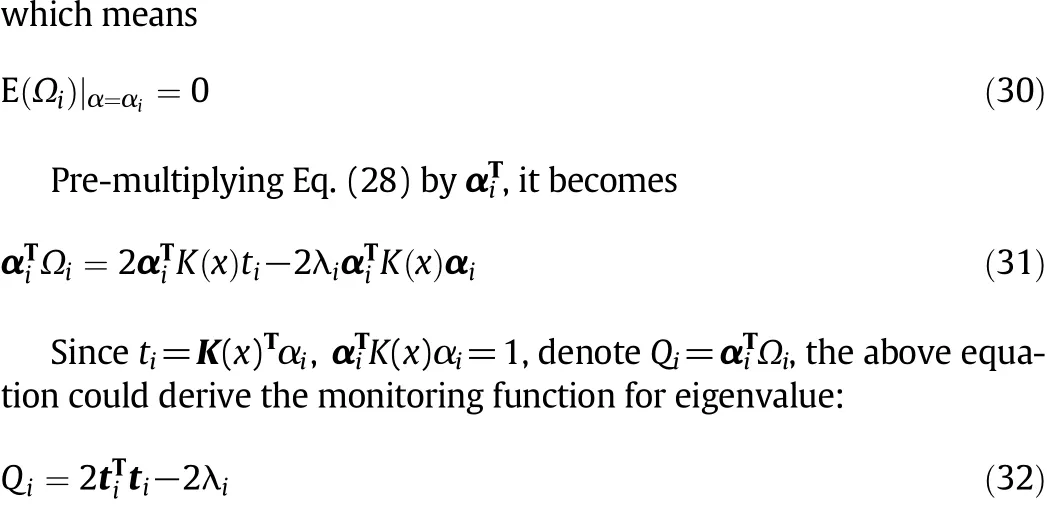
Then the monitoring function for the eigenvalue change could be developed with the score vector.The derivation is given in Appendix 1.Finally the eigenvalue change monitoring function satisfies the following equation:

where tiis the ith score vector obtained from Eq.(6)and λiis the ith eigenvalue of covariance matrix in feature space.Qiis the monitoring function for the ith eigenvalue.Then the residual vector ζ could be obtained from the monitoring function.

where Q is the monitoring function for all eigenvalues and its ith column of is Qi.λ denotes the eigenvalue.The ability of process monitoring for the residual vector ζ is investigated with the sufficiency given in Theorem 1.The proof of Theorem 1 is given in Appendix 2.

Theorem 1.If the process is in normal condition,the mean value of residual vector ζ is zero;otherwise it changes to a non-zero value.Thus,the process condition can be identified by a change on the mean value of ζ.

3.Incorporating Multivariate Time Delay Analysis into LKPCA

The key of the proposed fault prognosis model in this paper is incorporating multivariate time delay analysis into LKPCA monitoring.Through this method,the correlation degree is acquired through mutual information estimation and then the multivariate correlated time series can be developed as the input of BP network.BIC is used to calculate the time delay among multi-variables,and then the multivariate time delayed series can be constructed.As a monitoring approach,LKPCA construct two statistics for process monitoring in a moving window with the establishment of multivariate time delayed series and future values by BP.The flow diagram of the approach is depicted in Fig.1.

3.1.Get multivariate time delayed series

BIC is an un-supervised learning algorithm which can seek an optimal balance between model complexity and descriptive power for the model[28,29].For time delay estimation,BIC could determine the delay of time series model through achieving the minimum of the criterion.Assume the time series{xi}satisfies the following equation.

where xi(t),xi(t?1),xi(t?2),...,xi(t?tdi)separately denotes the ith process variable value at sample time t,t?1,t?2,...,t?tdi,φ1,φ2,...,φtdiis the weighted coefficient of xi(t?1),xi(t?2),...,xi(t?tdi)and e is a white noise following Gaussian distribution N(0,α).tdiis the delay of time series{xi}.Moreover,suppose the posterior probability function of time series{xi}is f(·|tdi),(tdi=1,2,...).The task of BIC is to get the proper value of time delay and then the approximation of the real time delayed series model is estimated.The definition of BIC is as follows.

In this way,the time delay td1,td2,...,tdmof all process variables is acquired.Therefore,the conventional multivariate time series x(t)=(x1(t),x2(t),...,xm(t))can be transformed into the multivariate time delayed series

3.2.Multivariate correlated time series prediction

In order to achieve prediction,time series prediction by BP network is applied.Moreover,to reflect the complex internal relationship among process variables,the input of BP network is set to be the multivariate correlated time series other than the original time series.The output of BP network is a series of future values of the process variable.Now take the jth variable as an example to illustrate the procedure of developing a BP network.

Firstly,mutual information estimation is used to acquire the correlation degree among process variables.The detailed procedures have been described in Section 2.1.Store the correlation degree into a matrix and then denote the matrix as R(R∈Rm×m)which is a symmetrical mutual information matrix.

Secondly,a binary matrix B is developed to clearly identify whether the process variables are correlated or not.If the element rijsatisfies rij＞θ×rjj,where θ(θ∈[0,1])is the threshold and riiis the self-mutual information,it means that variable i and variable j are strongly correlated and the element bijis denoted by“1”.Otherwise,the two variables show weak correlation and bijis denoted by “0”.The threshold θ is depended on the variable dimension and computation complexity.If the variable dimension is low or the demand of computation complexity is not relatively strict,to reduce the probability of deleting related variables the threshold θ is set to be a lower value and vice versa.Eq.(12)depicts the form of the binary matrix B.

Fig.1.Flow diagram of multivariate time delay analysis based LKPCA fault prognosis approach.

Thirdly,construct the multivariate correlated time series for the jth variable.Eq.(12)indicates that the jth process variable is related to three process variables(the ith process variable,the jth process variable and the kth process variable).So the multivariate correlated time series of the jth process variable is Svarj=(xi(t),xj(t),xk(t)).

Fourthly,construct a BP neural network for the jth variable.The input node number is decided upon the number of correlated variables and the output node number is determined by the prediction step.

Finally,train the net work.When the mean squared error reaches the minimum or the iteration number reaches the maximum,network training is regarded complete and the weights are fixed.

According to the steps above,the network is established well with the ability of simulating the nonlinear function between input and output.The structure of the jth BP network is shown in Fig.2 and the prediction step is three in this network.

Fig.2.BP Network structure of the jth variable.

3.3.Develop LKPCA incipient fault prognosis model

In this study,LKPCA is applied as the incipient fault prognosis model with the residual vector.Rewritten Eq.(9)as follows

Incorporating of time delayed series S(i)=(x1(i+td1),x2(i+td2),...,xm(i+tdm))and future values generated by BP denoted as x_pre(j)=(x1(j),x2(j),...,xm(j)),Eq.(13)is transformed as follows:

where tdmax=max{td1,td2,...,tdm}denotes the maximum time delay of all process variables.pre_step describes the prediction steps of BP network.To further increase sensitivity in detecting incipient fault,a moving window is used to reduce the computation burden.The residual is improved as follows:

whereare the covariance matrix of systematic and noisy part.Since the improved residual vector follows Gaussian distribution,the two statistics T2and SPE follows χ2distribution[23].The confidence limits of the two statistics T2and SPE can be determined by χ2distributed function and they are generally set as 95%or 99%.Through observing whether the statistics T2or the statistics SPE exceed the limit or not,it can be distinguished that the condition is normal or abnormal.

4.Case Study

To test the performance of multivariate time delay analysis based LKPCA fault prognosis approach,it is exemplified on a simple nonlinear process and TE benchmark process.Three methods are employed to compare the performance and they are separately multivariate time delay analysis based LKPCA(MTD_LKPCA),multivariate time delay analysis based KPCA(MTD_KPCA)and LKPCA.The fault detection accuracy(FDA)and false alarm rate(FAR)are used to evaluate the performance of these methods.The definition is as below:

whereand SPEthdenotes the threshold for statistic T2and statistic SPE.f≠0 and f=0 represents the fault and normal condition,respectively.

4.1.A simulated nonlinear process

There are three variables in the nonlinear process which are as follows:

where t∈[0.01,2],and e1,e2,e3∈N(0,0.01)are independent noise.300 samples are generated by Eq.(22)as normal data.Then twokinds of 300 artificial fault samples are separately generated as follows:

Table 1 FDA and FAR comparison result of simulated process

(1)Fault 1:A step bias of x2by?1 from the 101st sample.

(2)Fault 2:A ramp change of x1by adding 0.05(k?100)from the 101st sample.k denotes the sample number in the time series.

With the generated normal data,BIC is firstly applied to get the time delay of the three process variables and the results are3samples,2samples and 2 samples respectively.Therefore,the corresponding multivariate time delayed series is S(t)=(x1(t+3),x2(t+2),x3(t+2)).Then the correlation among process variables is under review by mutual information estimation.In this study,the relevant tuning parameter k and the threshold θ are separately set to be 30 and 0.05.The experimental results indicate that the process variables are all correlated with each other.It also could be inferred from Eq.(22).Hence,the input node number of the three BP network predictors is three.Moreover,the input for mis S(t)=(x1(t),x2(t),x3(t))and the combination of all BP net work predictors output is x_pre(t+1)=(x1(t+1),x2(t+1),x3(t+1)).

For incipient fault prognosis,two statistics in the LKPCA model are calculated using Eq.(15)with the multivariate time delayed series S(t)=(x1(t+3),x2(t+2),x3(t+2))and prediction series x_pre(t+1)=(x1(t+1),x2(t+1),x3(t+1)).The length of moving window is selected to be 35 and statistical confidence limits of statistic T2and statistic SPE are set to be 99%.The experimental results of MTD_KPCA,LKPCA and MTD_LKPCA with the in dices FDA and FAR are listed in Table 1.

Table 2 Process Faults of TE Process

From Table 1,it is noted that with MTD_KPCA method,the statistic T2couldn't violate the threshold at all and the fault detection accuracy of statistic SPE is very low.However, in applying LKPCA and MTD_LKPCA method,the fault detection accuracy of statistic T2greatly improved.The performance results from the incorporation of high sensitive LKPCA.Moreover,through comparing MTD_LKPCA and LKPCA,it can be seen that MTD_LKPCA has higher FDA and lower FAR than LKPCA no matter on fault 1 or fault 2.The better experimental results of MTD_LKPCA show the proposed approach is meaningful and more effective on incipient fault prognosis compared to the original LKPCA method.

4.2.TE benchmark process

TE benchmark process provides a practical industrial nonlinear process which has been widely used to test the performance of various fault diagnosis and prognosis approaches[30].It consists of five major unit operations:a reactor,a condenser,a compressor,a separator and a stripper.The flow diagram of the process is shown in Fig.3.

Fig.3.Flow diagram of the TE process.

Table 3 Process measurements of TE process

This process has 20 programmed faults which are listed in Table 2.Among them,fault 3 and fault 9 are not easy to be detected by most methods duo to their little change on variables from normal condition[31,32].In the paper[31],it points out that most data-driven process monitoring methods give low fault detection rate thus cannot detect the faults successfully.In the paper[32],the experimental results also show that fault diagnosis using singe neural network(SNN)or multilayer perceptron(MLP)network cannot detect these two faults at all.

The TE process consists of 41 measured variables which are listed in Table 3.In this experiment,all measured variables are used to show the performance of three methods.All 21 runs(one normal and 20 fault runs)are performed for 48 h and the sampling interval is set to be 3 min.

4.2.1.Experimental results

BIC is firstly used to acquire the time delay and then mutual information estimation is applied to calculate the correlation degree.In this experiment,the tuning parameter k and the threshold θ in mutual information estimation are selected to be 50 and 0.2 respectively. The experimental results for TE process are listed in Table 4.With the time delay and correlation information, the multivariate time delayed series and multivariate correlated time series can be developed.

For multivariate time series prediction,BP network predictor for each process variable is constructed whose input could be determined by the correlated variables.To generate training and test dataset,one normal condition and 20 fault conditions are performed.All fault simulation runs started in normal condition while introduces faults after six simulation hours.For generating training dataset,the sampling interval is set to be 15 min.For each fault pattern,the first 24 observations are under normal condition,which are discarded.The remaining data are taken as the training data.For generating test dataset,the sampling interval is set to be 3 min.Thus,for each pattern the total number of test dataset is 960.

In the LKPCA model,two statistics are constructed for fault prognosis in a moving window with the multivariate time delayed series andprediction series by BP network. Here, the length of the moving window is selected to be 50 and the statistical confidence limits of statistic T2and statistic SPE are set to be 99%.

Table 4 BIC and MI experimental results for TE process

Fig.4.Monitor result of MTD_KPCA on TE process fault 3.

4.2.2.Comparison results

To test the sensitivity of the proposed approach,fault 3 and fault 9 are used.For each fault pattern,the introduction is at sample 121.As the length of the moving window is set to be 50,the fault can be detected at the 71st window.The monitoring results of MTD_KPCA,LKPCA and MTD_LKPCA for fault 3 are separately given in Fig.4-6.From Fig.4,it can be seen that MTD_KPCA cannot detect the fault 3 since there is no threshold violation either by statistic T2or SPE.However,the fault prognosis performance of LKPCA and MTD_LKPCA are greatly improved due to the incorporation of statistical local approach.In Fig.5,the fault 3 can be detected at the 104th window by LKPCA with the SPE statistic exceeding the threshold.However,in Fig.6 MTD_LKPCA could detect the fault 3 at the 92nd window which is much earlier than LKPCA method.

Fig.5.Monitor result of LKPCA on TE process fault 3.

Fig.6.Monitor result of MTD_LKPCA on TE process fault 3.

For fault 9,the monitoring results of MTD_KPCA,LKPCA and MTD_LKPCA are separately given in Fig.7-9.It can be seen from Fig.7 that MTD_KPCA cannot detect fault 9 since there is no threshold violation either by statistic T2or SPE.In Fig.8,fault 9 can be detected at the 116th window by LKPCA.For MTD_LKPCA,seen from Fig.9,it is detected at the 96th window which shows much better on the detection response.The difference between MTD_LKPCA and LKPCA mainly derives from the incorporation of multivariate time delay analysis,which could re fl ect the complete information of the current condition.For further revealing the performance of MTD_LKPCA,the corresponding FDA and FAR comparison results for the three methods are listed in Table 5.

From Table 5,it can be seen that FDA of the proposed method is higher than MTD_KPCA and LKPCA method no matter what the prediction steps are.Also,for MTD_LKPCA,the FDA will be lower with more prediction steps. If the long prediction steps are needed,more prediction steps can be selected.If the accuracy is strict,fewer prediction steps can be selected.Moreover,the FAR of MTD_LKPCA is obviously lower than MTD_KPCA and LKPCA whatever the prediction steps are.It is noted that there will be no false alarm rate with more prediction steps.Above all,MTD_LKPCA is a much better method than MTD_KPCA and LKPCA on the aspect of fault response,FDA and FAR.

Fig.8.Monitor result of LKPCA on TE process fault 9.

Fig.9.Monitor result of MTD_LKPCA on TE process fault 9.

Table 5 Comparison results of FDA and FAR for TE process

5.Conclusions

This paper has proposed a new integrated multivariate time delay analysis and LKPCA based fault prognosis method for nonlinear processes.In this method,mutual information estimation and BIC are used to acquire the correlation degree and calculate the time delay among multi-variables.In order to achieve prediction,BP network is established as the approach to multivariate correlated time series prediction.For further fault prognosis,two statistics in the LKPCA model are constructed with the establishment of multivariate time delayed series and prediction series by BP.The new method is exemplified on a simple nonlinear and the TE benchmark process compared with LKPCA and MTD_KPCA.The experimental result shows that this new method could prognosis incipient fault and has higher fault detection accuracy.Therefore,this new method seems to be an efficient fault prognosis method than the existing work.

Appendix 1.Proof of monitoring function for eigenvalue

Commencing with the formulation of the ith eigenvector on the following optimization function:

Appendix 2 Proof for Theorem 1

Denote the ith eigenvalue and kernel matrix in normal condition as λiand K(x),the departure of λiand K(x)are separately denoted as△λiand△K(x),thus

Therefore,the monitoring function Qisatisfies Qi=0,if the process is in normal condition and Qi≠0,if the process is in abnormal condition.Notice Eq.(9),the residual vector ζ is derived from the monitoring function.It also satisfies ζ=0,if the process is in normal condition and ζ≠0,if the process is in abnormal condition.

[1]D.Bustan,N.Pariz,S.K.Hosseini Sani,Robust fault-tolerant tracking control design for spacecraft under control input saturation,ISA Trans.53(2014)1073–1080.

[2]S.Ahmet,J.Sarangapani,S.Can,Mahalanobis–Taguchi system as a multi-sensor based decision making prognostics tool for centrifugal pump failures,IEEE Trans.Reliab.60(2011)864–8708.

[3]J.Chen,H.Sheng*,C.Li,Z.Xiong,PSTG-based multi-label optimization for multi-tracking,Comput.Vis.Image Underst.144(2016)217–227.

[4]K.Ashwani,A.P.Singh,Fuzzy classifier for fault diagnosis in analog electronic circuits,ISA Trans.52(2013)816–824.

[5]B.Chen,P.C.Matthews,P.J.Tavner,Wind turbine pitch faults prognosis using A-priori knowledge-based ANFIS,Expert Syst.Appl.40(2013)6863–6876.

[6]M.Basseville,On-board component fault detection and isolation using the statistical local approach,Automatica 34(1998)1391–1415.

[7]H.Chang,J.H.Chen,Y.P.Ho,Batch process monitoring by wavelet transform based fractal encoding,Ind.Eng.Chem.Res.25(2006)3864–3879.

[8]L.Zhang,Fault prognostic algorithm based on multivariate relevance vector machine and time series iterative prediction,Procedia Eng.29(2012)678–686.

[9]G.Li,S.J.Qin,Y.D.Ji,D.H.Zhou,Reconstruction based fault prognosis for continuous processes,Control.Eng.Pract.18(2010)1211–1219.

[10]T.Jo,VTG schemes for using back propagation for multivariate time series prediction,Appl.Soft Comput.13(2013)2692–2702.

[11]C.H.Gao,Z.M.Zhou,J.M.Chen,Assessing the predictability for blast furnace system through nonlinear time series analysis,Ind.Eng.Chem.Res.47(2008)3037–3045.

[12]M.S.Roulston,Estimating the errors on measured entropy and mutual information,Phys.D 125(1999)285–294.

[13]G.Chen,L.Xie,J.S.Zeng,J.Chu,Y.Gu,Detecting model-plant mismatch of nonlinear multivariate systems using mutual information,Ind.Eng.Chem.Res.52(2013)1927–1938.

[14]B.Sadeghi,HM.A BP-neural network predictor model for plastic injection molding process,J.Mater.Process.Technol.103(2000)411–416.

[15]W.X.Zhao,D.Z.Chen,S.X.Hu,Detection of out lier and a robust BP algorithm against outlier,Comput.Chem.Eng.28(2004)1403–1408.

[16]J.F.B?hme,Time delay estimation by cross-covariance maximization of quadrature sampled narrow band signals,AEU Int.J.Electron.Commun.58(2004)13–20.

[17]S.H.Jin,P.Lin,M.Hallett,Linear and nonlinear information flow based on time delayed mutual information method and its application to corticomuscular interaction,Clin.Neurophysiol.121(2010)392–401.

[18]W.D.Penny,Comparing dynamic causal models using AIC,BIC and free energy,Neuroimage 59(2012)319–330.

[19]M.A.Kramer,Nonlinear principal component analysis using auto-associative neural networks,AIChE J.37(1991)233–243.

[20]J.Wang,H.T.Wei,L.L.Cao,Q.B.Jin,Soft-transition sub-PCA fault monitoring of batch process,Ind.Eng.Chem.Res.52(2013)9858–9888.

[21]J.M.Lee,C.K.Yoo,S.W.Choi,P.A.Vanrolleghem,I.B.Lee,Nonlinear process monitoring using kernel principal component analysis,Chem.Eng.Sci.59(2004)223–234.

[22]J.M.Lee,C.Yoo,I.B.Lee,Fault detection of batch processes using multi way kernel principal component analysis,Comput.Chem.Eng.28(2004)1837–1847.

[23]Z.Q.Ge,C.J.Yang,Z.H.Song,Improved kernel PCA-based monitoring approach for nonlinear processes,Chem.Eng.Sci.64(2009)2245–2255.

[24]U.Kruger,S.Kumar,T.Littler,Improved principal component monitoring using the local approach,Automatica 43(2007)1532–1542.

[25]Z.Q.Ge,L.Xie,U.Kruger,Z.H.Song,Local ICA for multivariate statistical fault diagnosis in systems with unknown signal and error distributions,AIChE J.58(2012)2357–2372.

[26]A.Kraskov,H.St?gbauer,P.Grassberger,Estimating mutual information,Phys.Rev.E 69(066138)(2004).

[27]S.Markus,R.Haber,U.Schmitz,Source identification of plant-wide faults based on k nearest neighbor time delay estimation,J.Process Control 22(2012)583–598.

[28]Y.Shi,W.Q.Meeker,Bayesian methods for accelerated destructive degradation test planning,IEEE Trans.Reliab.61(2012)245–253.

[29]F.A.Carroll,J.M.Godinho,F.H.Quina,Development of a simple method to predict boiling points and fl ash points of acyclic alkenes,Ind.Eng.Chem.Res.50(2011)14221–14225.

[30]A.Singhal,D.E.Seborg,Evaluation of a pattern matching method for the Tennessee Eastman challenge process,J.Process Control 16(2006)601–613.

[31]Y.Shen,S.X.Ding,A.Haghani,H.Y.Hao,P.Zhang,A comparison study of basic data-driven fault diagnosis and process monitoring methods on the benchmark Tennessee Eastman process,J.Process Control 22(2012)1567–1581.

[32]R.Eslamloueyan,Designing a hierarchical neural network based on fuzzy clustering for fault diagnosis of the Tennessee–Eastman process,Appl.Soft Comput.11(2011)1407–1415.