EVALUATION OF ADDED RESISTANCE OF KVLCC2 IN SHORT WAVES*

GUO Bing-jie, STEEN Sverre

Department of Marine Technology, Norwegian University of Science and Technology, NO-7491 Trondheim, Norway, E-mail: bingjie.guo@ntnu.no

EVALUATION OF ADDED RESISTANCE OF KVLCC2 IN SHORT WAVES*

GUO Bing-jie, STEEN Sverre

Department of Marine Technology, Norwegian University of Science and Technology, NO-7491 Trondheim, Norway, E-mail: bingjie.guo@ntnu.no

(Received April 11, 2011, Revised July 7, 2011)

The added resistance of KVLCC2 in short and regular head waves has been studied theoretically and experimentally. Model tests are performed to determine how well the asymptotic formula (Faltinsen et al. 1980) predicts the typical level of added resistance in short waves. Because the asymptotic formula neglects the effects of ship motions, it is combined with theoretical methods to calculate the added resistance in long waves using an R function to predict the added resistance in the intermediate wavelength region where both ship motions and wave reflection are important. A unique feature of this experiment is that the ship model is divided into three segments to explore the added resistance distribution with respect to hull segment. This paper discusses the sensitivity of experimental results to the quality of the incident regular head waves. Moreover, a novel procedure for analyzing added resistance is described. Finally, the experimentally determined added resistance of KVLCC2 is compared with theoretical results. It is shown that the added resistance from the combined theoretical methods agrees well with experimental results in both the intermediate and short wave regions. The use of hull segments shows that added resistance is concentrated primarily at the bow.

added resistance, KVLCC2, short waves, R function

Introduction

Added resistance in short waves is an important factor in a large ship’s performance, because most of the time a large ship travels in small sea states[1], and the ability to sustain speed in a seaway is one of the primary objectives in the design of ships. International Towing Tank Conference (ITTC) standard procedure requires an estimate of the added resistance in waves for the calculation of sea margins, but does not specify a particular method[2]. The new Ship Performance Index (SPI) proposed by International Maritime Organization (IMO) includes the added resistance in waves, but for the prediction of added resistance in short waves, this index requires model tests “or an equivalent formula with considerable accuracy”[3].

Ship motions in short waves are negligible, and the added resistance in short waves is primarily due to wave reflection. Fujii and Takahashi provided a formula for ship resistance increase due to wave reflection at the ship bow. In their theory, Havelock’s formula for drift force based on the wave reflection was used together with empirical corrections[4]. Faltinsen et al. derived an asymptotic formula to calculate the added resistance of conventional displacement vessel in short waves. His formula is notable for taking into account the interaction of diffraction waves with steady current around the hull, although this is accomplished in an approximate way. When estimating the added resistance of a full hull form with Faltinsen’s asymptotic formula, Sakamoto and Baba recommended using the double body flow velocity around the waterline, instead of the approximate velocity V used by Faltinsen[5]. Admittedly, modifications and improvements to Fujii and Takahashi’s formula have been considered by several authors, such as Sakamoto and Baba, Matsumoto et al.[6]. However, none of the modifications provide added resistance that is significantly different from that by Faltinsen’s asymptotic formula. Furthermore, it is difficult to explain the physical meaning of empirical correction factors, because Fujii and Takahashi’s formula is a semi-empirical formula, whereas the asymptotic formula given by Faltinsen is directly derived from a simplified physical model. Therefore, in this study, a theoretical estimate of the added resistance for an advancing displacement ship in short waves is carried out using the asymptotic formula from Faltinsen et al..

Model tests of added resistance in short waves are very difficult to perform due to the instability of short waves and experimental uncertainty. An experiment on large full ships in short waves was performed by Wada and Baba. Three ship models with different principal dimensions and bow bluntness were tested. The results show that the improved asymptotic formula from Sakamoto and Baba underestimates the added resistance and that the added resistance mainly depends on the shape of the waterline in the vessel’s fore region[6]. An experiment performed by Steen and Faltinsen[7]using different types of displacement ships indicated that the stability of short waves is the main source of experimental error. The experiment is used to verify Faltinsen’s asymptotic formula, and the results show that this formula underestimates the experimentally measured added resistance. Recently, two models (a container ship and a pure car carrier) in short waves were studied by the Japanese National Maritime Research Institute[8], and the results show that the conventional Fujii and Takahashi’s formula without the correction from Tsujimoto underestimates the added resistance in short waves. For KVLCC2 ship model, several experimental studies in calm water have been performed[9,10]. However, a sea-keeping test of this model was not performed until 2010[11]. At the Gothenburg 2010 Workshop, Osaka University and INSEAN presented the results of sea-keeping tests, but their tests focused on three long waves. The experiment presented in this paper focuses on the added resistance in the short and intermediate wavelength regions, an analysis of the resistance distribution along the hull is also presented.

The purpose of this study is to validate Faltinsen’s asymptotic formula and its application range, to find a better method with which to calculate the added resistance in waves with an intermediate wavelength (1 ＜ L/λ＜ 3). Considering the difficulties associated with added resistance experiments in short waves, the sensitivity of the results to the quality of the waves is discussed in this paper, and new approaches for analyzing the measured wave amplitudes and added resistance are proposed. As for the theoretical calculation, two combination methods with different numerical approaches are explored to estimate the added resistance in intermediate waves: a combination of the asymptotic method and the Radiated Energy Method (REM) with strip theory, and a combination of the asymptotic method and the radiated energy method with the “modified” pressure integration method (G & B). Finally, comparisons of the added resistance in incident regular head waves of KVLCC2 from the experiment and from the combination calculations at selected Froude numbers are analyzed.

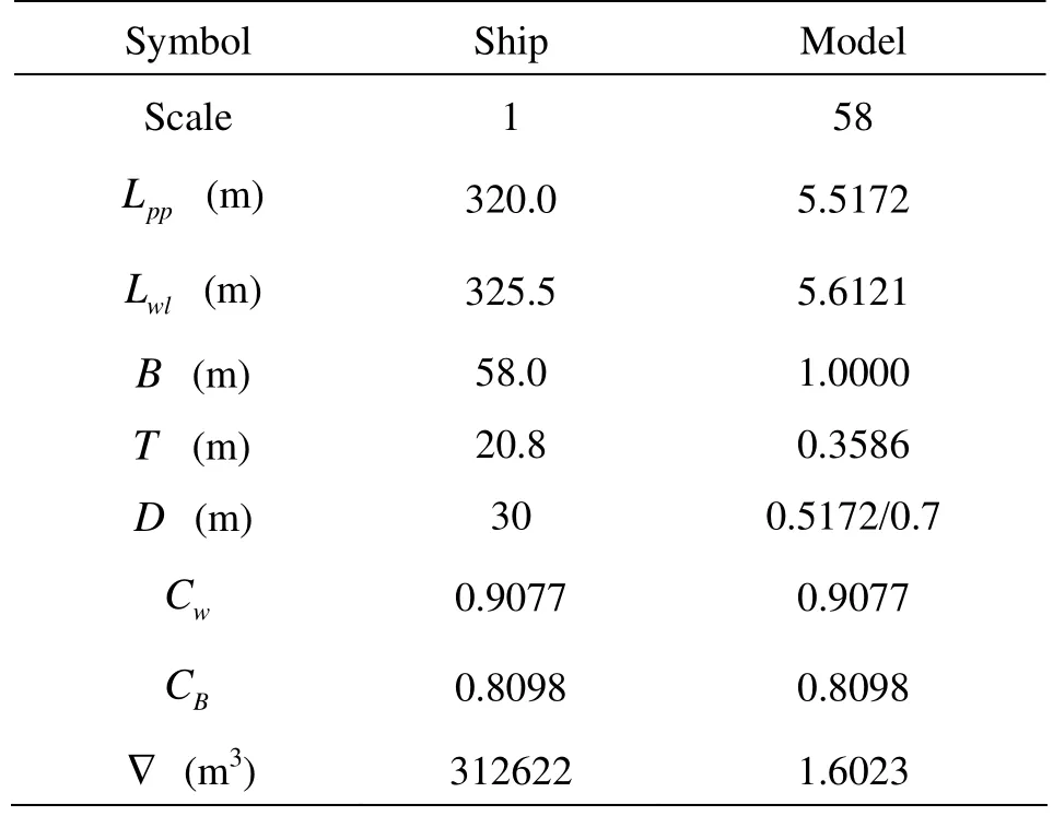
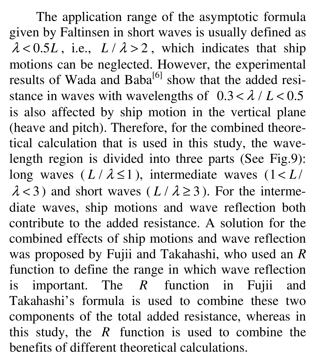
Table 1 Main dimensions of KVLCC2

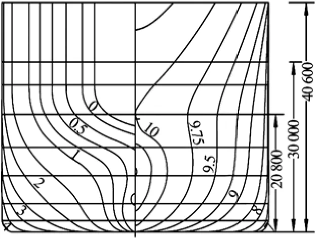
Fig.1 Body plan of the experimental model (dimensions in mm full scale)

1. Experiment

1.1 Model test

A segmented model of the MOERI (Maritimeand Ocean Engineering Research Institute) KVLCC2 tanker was built at MARINTEK. The model is a hull and is not equipped with either a rudder or a propeller. The main dimensions are shown in Table 1, and a detailed description is provided in SIMMAN (2008)[12]. For the sea-keeping test, the designed ship depth is too small to prevent water on the deck. Thus, the depth is increased to 0.7 m through the extrapolation of the frame lines. The body plan of the experimental model is shown in Fig.1.

The model is divided into three segments: foresegment, aft-segment, and the parallel mid-body. An aluminum frame is used to keep the three segments together. The fore- and aft-segments are connected to the frame through springs and force transducers. The springs only absorb vertical forces, whereas the force transducers measure the longitudinal forces. Motion between the segments is very limited, thus, the model is a good approximation of a rigid model.

Fig.2 Dimensions in mm model scale of each segment and the friction plate

The model is connected beneath the towing carriage using a connection system that is normally used for calm water towing tests. The model is connected to the carriage by a towing force dynamometer. The location of the external towing force is shown in Fig.2. To avoid overloading the towing force dynamometer as a result of carriage speed variations, a flexible connection is used between the model and the dynamometer. There is also some flexibility in the fixture of the towing force dynamometer. To avoid resonant surge motion caused by the flexible connection during the measurements, the natural period of surge TNis measured with a decay test. The measured TN=4.26s is not close to the wave encounter periods used in the test.

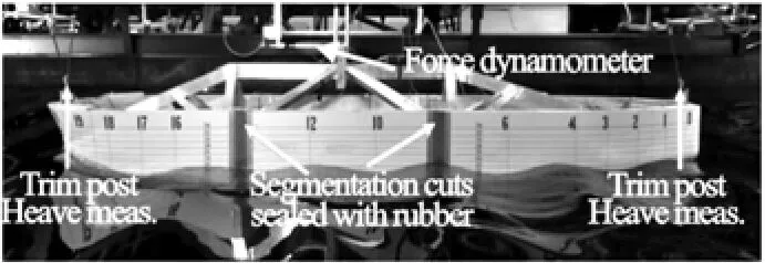
Fig.3 Experimental set-up

In this set-up, the model is also connected to the carriage by trim posts at the fore and aft perpendiculars. The trim posts allow freedom in heave and pitch, but keep the model fixed in sway and yaw. The surge motion is limited. Vertical motion is measured at the trim posts. The connection of the model to the carriage is illustrated in Fig.3. A friction plate that was used to measure the local frictional force is shown in Fig.2. For measuring undisturbed wave elevation, two acoustic wave meters are placed on the towing carriage to measure the wave elevation in front of the model, and another two conductive wave meters are placed close to the wave maker to measure the wave elevation in the towing tank.

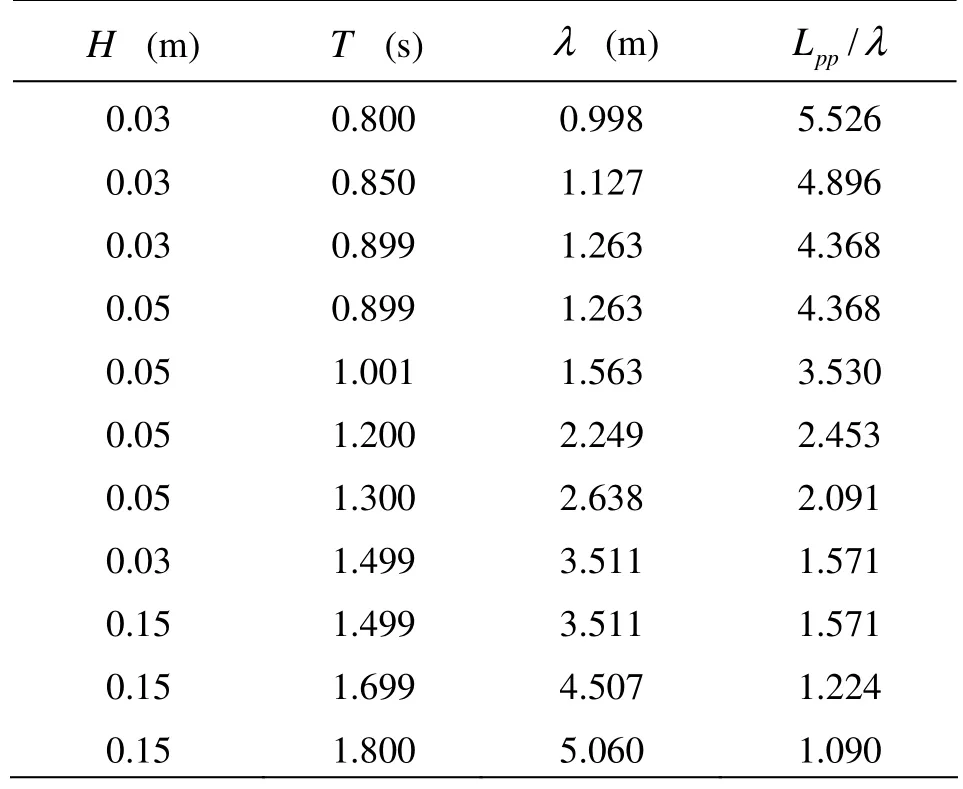
Table 2 Regular waves applied in the tests

The experiment is conducted in regular head waves of different lengths and amplitudes. The wavelength λ ranges from 0.181Lppto 0.917Lpp, and the wave height H ranges from 0.03 m to 0.15 m. The waves used in the tests are shown in Table 2. Five Froude numbers were tested: Fr=0, 0.05, 0.09, 0.142 and 0.18, where Fr =0.142 corresponds to the design speed.

1.2 Experimental analysis

The model test was conducted in the large towing tank ( L×B×D =260 m × 10 m × 5 m ) at the Marine Technology Centre in Trondheim, Norway. The test procedure that was used for all cases was to run the model in calm water for the first part of the run down the tank to determine the calm water resistance, and then have the model encounter the regular wave train to obtain the resistance in waves. The added resistance was then found by taking the difference in mean resistance between the two parts of the run. This procedure was used to minimize the experimental uncertainty caused by occasional drifts or changes in the resistance measurement.

1.3 Wave calibration

The measurement of added resistance in short waves is very difficult, primarily due to the instability of short waves and their small amplitudes. Previousexperiments have shown that errors in the measurements are primarily due to unstable waves and their related effects[13].

Waves with high steepness are unstable (called the Benjamin-Feir instability effect), and short waves with low steepness are subject to more spatial variation than long waves due to the variation in their transversal amplitude across the tank[14]. For this issue, the waves are calibrated at the beginning of the experiment. The calibration is performed after suitable wave steepness and stable propagation range are selected, which ensures that the short waves are stable over the expected range (approximately 80 m) in the towing tank.

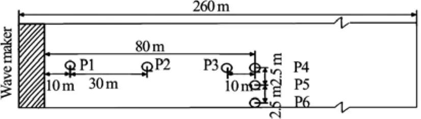
Fig.4 Position of wave probes during wave calibration

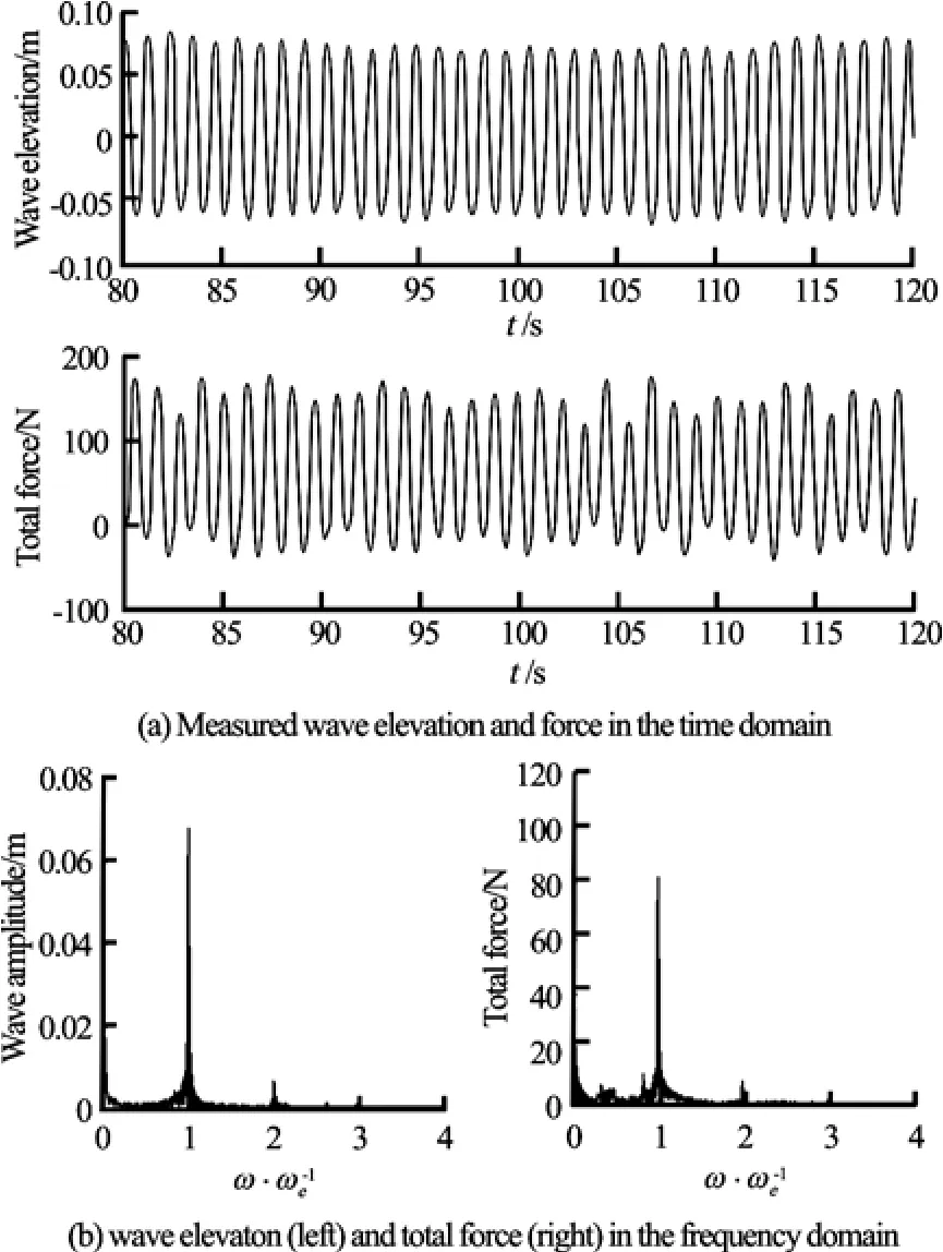
Fig.5 Wave and total resistance measurement

The calibration approach uses the configuration shown in Fig.4, where six wave probes are distributed down the middle and from the side of towing tank. The experiment is only conducted with the wave if its elevation measured by these six wave probes is stable. Wave amplitude decreases slightly along the propagation distance. To minimize the effect of this phenomenon on the added resistance coefficient, the added resistance is made dimensionless using the square of the undisturbed wave amplitude, which is measured by a wave probe on the carriage.

1.4 Force analysis

In addition to the wave stability issue, the accuracy of the measurements is also a critical issue. Data post-processing is used to reduce the uncertainty in the measurements. As shown in Fig.5(a) (the lower half of the figure), the total resistance in the waves oscillates not only with the wave encounter frequency but also with a lower frequency. The Fourier Transform (FT) results for the measured wave and the total force are shown in Fig.5(b). The wave measured by the wave probe on the carriage has a very low frequency component because the rail of the towing tank rises slightly towards the end of tank.

The FT result for the total force shows that low frequency noise also exists. Possible reasons for the existence of this noise in the total resistance measurement include the 2nd order wave force, the uncertainty in the wave generation by the wave maker (low frequency wave component), and the disturbance from the carriage through the elastic connection between the carriage and model.

To eliminate the influence of this low frequency resistance variation on the added resistance, the added resistance coefficient is calculated using a new data processing method. The fluctuation of the measurement data is expressed as the sum of a stable value, a value oscillating with the encounter frequency and a value oscillating at a low frequency (“noise”). To eliminate the “noise” effect, the start and end points are randomly selected many times within the observed period of “noise” as:

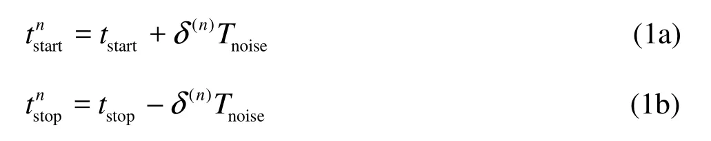
where tstartand tstopare the start and end time of the selected measurement data, which are selected by visual inspection of the time series. tnand tn

startstopare the randomly chosen start and stop point of the n-th time window. δnis the n-th random number uniformly distributed at [0,1]. Tnoiseis the observed period of the “noise”.

The added resistance of the n-th time window R(n)is then given as

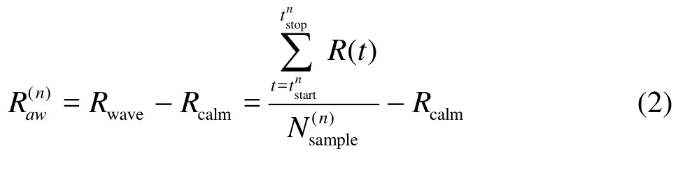
awwhere R( t) is the measured resistance in waves at each sample time, and N(n)is the sample number

sample in the n-th time window. Rcalmis the ship resistance in calm water, which is calculated in the same way as the average resistance in waves Rwave.

Then, the wave amplitude in the n-th time window ζa(n)is calculated in the same way as

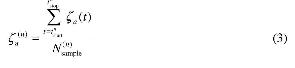
n

where ζa(t) is the measured wave amplitude at each sample time.

Finally, the average dimensionless added resistance coefficient Cawis expressed as

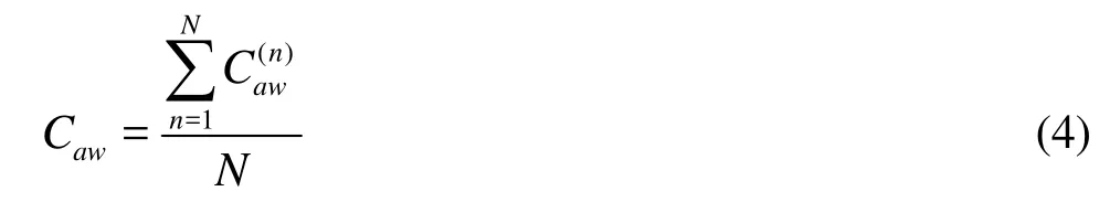
where C(n)=R(n)/ρ g ζ(n)2B2/L is the added resi

aw aw a pp stance coefficient calculated in the n-th time window, B and Lpprefer to Table 1, and N is the number of randomly selected time windows.

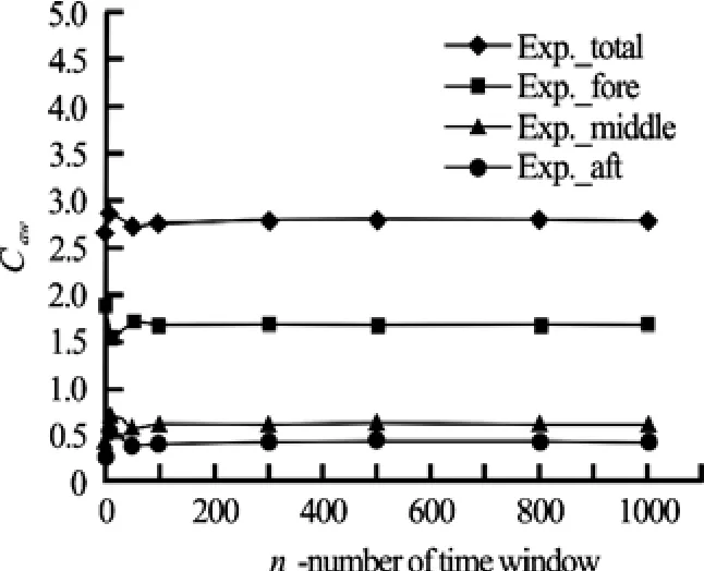
Fig.6 Effect of increasing number of time windows

The average value of added resistance coefficient vs. the number of time windows for one experimental case is shown in Fig.6, which shows that the added resistance coefficient stabilizes after approximately 300 time windows have been averaged. Thus, 1 000 time windows are used to process the experimental data in this study.

To validate this data processing method, one signal with low frequency noise is processed. The original signal is y = a1sin(2 π/Τ1t )+35, where a1=80 and T1=1.2s. To obtain a signal characteristic similar to that shown in Fig.5, the amplitudes and periods of low-frequency noises are carefully selected. The final signal is

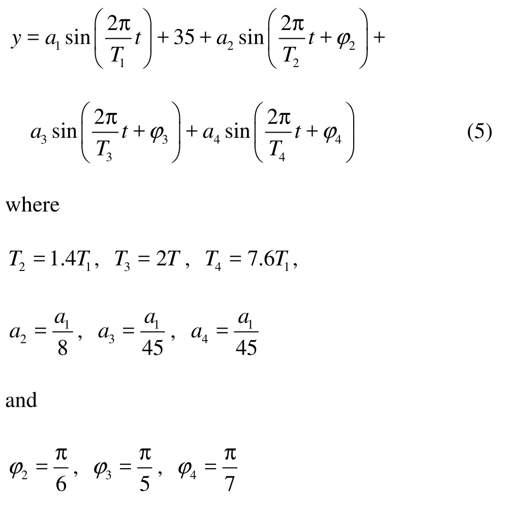
The final signal in both the time and frequency domains is shown in Fig.7.

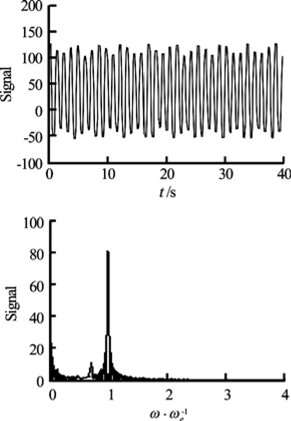
Fig.7 Simulated signal in the time and frequency domains

With the proposed data processing method, the period of noise is set as the period of strongest noise, i.e., Tnoise= T2. A single time window results in a mean signal value of y(0)=34.3792with an error of 1.78%, whereas 1 000 time windows results in a mean signal value of y(0)=35.0650with an error of 0.19%. These results indicate that the proposed data processing approach can achieve a highly accurate result for the mean value.

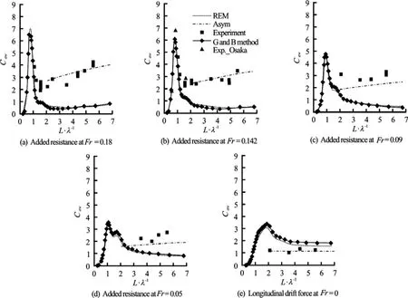
Fig.8 Added resistance comparison of experimental and theoretical results

2. Added resistance calculations

In this section, three theoretical methods are presented for calculating the added resistance, and their limitations are discussed. We consider a ship advancing at a constant mean forward speed in regular head waves. A right-handed coordinate system (x, y, z) fixed with respect to the mean oscillatory position of the ship is used. The z-axis is positive vertically upwards through the center of gravity of the ship. The x-axis is pointing towards the stern. The origin is located in the plane of an undisturbed free surface. The ship length L used for all of the calculations is Lpp.

2.1 Radiated energy method

2.1.1 Radiated energy method for added resistance

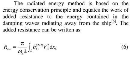
where b(2D)is the damping coefficient of vertical

33 motion at section xb, ωeis the encounter frequency, and λ is the wavelength. Vzais the amplitude of the vertical relative velocity Vz, which is a harmonic function.

The vertical relative water velocity Vzcan be approximated by

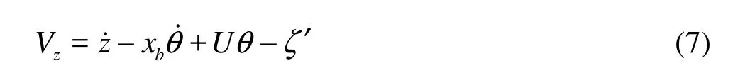
where θ is the pitch angle, z˙ is the ship’s vertical velocity, U is the ship forward speed, and ζ′ is the effective wave displacement for the cross-section xb, which is a correction to the Froude-Kryloff hypothesis. This correction affects the incident wave amplitude, and for deep water, it can be calculated by

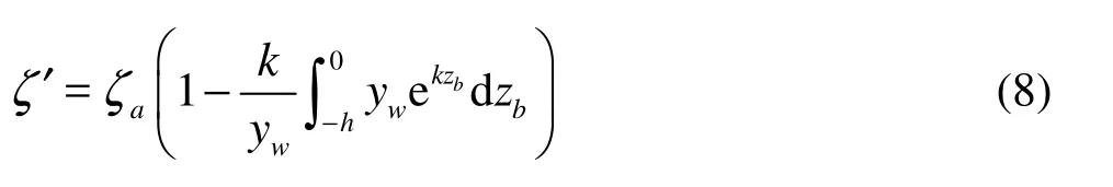
where k is the wave number, zbis the vertical coordinate at the body frame, h is the ship draft, ywis the half width of design waterline at section xband aζ is the wave amplitude without modification.

The value of the relative motion is important in this method. With accurate prediction of ship motions, this method works well in long waves. The ship motions can be corrected to include wave diffractionusing the empirical Eq.(8), but this correction does not provide satisfactory results, especially in short waves (See Fig.8).

2.1.2 Strip theory for ship motion

Knowledge of ship motions and hydrodynamic characteristics such as added mass and the damping coefficient is required to calculate the added resistance using the radiated energy method, according to Eq.(6). Strip theory is adopted to provide the necessary information here. Using the Salvesen-Tuck-Faltinsen (STF) method[5], the calculation is performed for a range of regular waves, where the hydrodynamic coefficients and motion amplitude are obtained for each frequency.

2.2 G & B method

This method is similar to the radiated energy method presented in Subsection 2.1. The only difference is that the “Modified” pressure integration is used for calculating ship motions, instead of the STF method.

“Modified” pressure integration is based on strip theory. In this method, the panels are distributed among each strip. By matching a near-field solution from the boundary element method with a far-field solution from asymptotic analysis, the radiation problem is solved. The added mass and damping coefficient are calculated with the STF method. The exciting loads, namely Froude-Kriloff and diffraction loads, are found by integrating the incident hydrodynamic pressure on the center of each panel and using the Haskind relation. Along with the hydrodynamic coefficient and the wave exciting loads, the ship motions in six degrees of freedom are calculated according to Newton’s 2nd law. The details can be found in Guo and Sverre[6].

2.3 Asymptotic formula

The asymptotic formula provided by Faltinsen[5]uses incident waves on an infinitely long vertical plane wall to simulate the diffraction problem in short waves. The wave reflection effect is included in the asymptotic formula without consideration of ship motion, which differs from the empirical correction of ship motion using the radiated energy method. The added resistance per unit length in head waves normal to the hull is written as

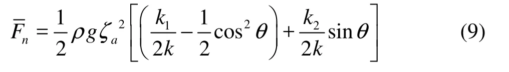
where ζais the wave amplitude, θ is the angle between the tangent of the waterline and x-axis, k is the wave number, k1=(ωe?Vk cosθ)2/g , V is the horizontal steady velocity parallel to the ship’s side and k2=k12? k2cos2θ.

With V = U cosθ , where U is the ship velocity, the added resistance along x-axis is

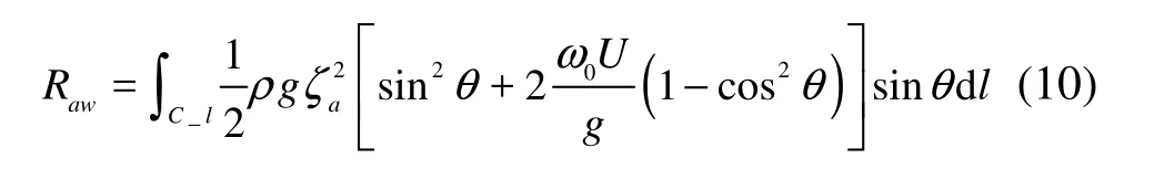
where ω0is the wave frequency, and the integration in Eq.(10) is performed along the non-shadow part C _l of the ship waterline curve as shown by Faltinsen et al.[5].

As mentioned above, this asymptotic formula is based on a simplified model of a ship in short waves and does not include radiated waves. The range of usage is moderate Froude number, i.e., Fr<0.2-0.25, a blunt ship bow and short waves, i.e.,L/λ＞2.

2.4 A comparison of the experimental and traditional theoretical results

The experimental results are compared with the theoretical calculations presented in the previous section. To clarify the notation when referring to Fig.8,“REM” represents the added resistance calculated with the radiated energy method (Subsection 2.1), “G & B method” represents the added resistance from “G & B” method (Subsection 2.2), and “Asym” represents the added resistance from the asymptotic formula (Subsection 2.3).

The only difference between “REM” and “G & B” methods is that the former calculates the ship motion using the “STF” method, whereas the latter uses “Modified” pressure integration. Figure 8 shows that the “REM” and “G & B” methods produce almost the same added resistance, which indicates that the“STF” method and “Modified” pressure integration predict almost the same ship motions in this case. This similarity occurs because “Modified” pressure integration is based on strip theory, and the panels are distributed among each strip. The physical parameters on the panels are calculated by interpolating between the strip lines.

The added resistance in long waves measured by Osaka University (2010)[11]is also presented in Fig.8(b). This figure shows that the theoretical methods can accurately predict the added resistance of KVLCC2 in long waves. Theoretical methods underestimate the added resistance at the peak area because non-linear effects are quite strong in this area, and the theoretical methods could not effectively model this region as a result.

Neither the radiated energy method nor the “G & B” method can accurately predict added resistance in short waves because they only adopt the empirical Eq.(8) to account for wave reflection. The asymptotic formula can accurately predict added resistance in short waves because it takes into account the interaction of diffraction waves with the steady current around the hull, although only in an approximate manner. However, its application region is limited to short waves, as it assumes that ship motions are negli-gible. Therefore, a new method is suggested here for predicting the added resistance in the wavelength region 1 ＜ L/λ＜ 3, where both ship motions and wave reflection provide an important contribution to added resistance.

3. Combined added resistance theory

The combined calculations for the added resistance are presented here. In this section, two different combinations of theories, denoted as the “REM” and“G & B” methods, are investigated. In the combined theory, the “REM” and “G & B” methods in Section 2 are combined with the asymptotic formula by an R function.

3.1 The R function

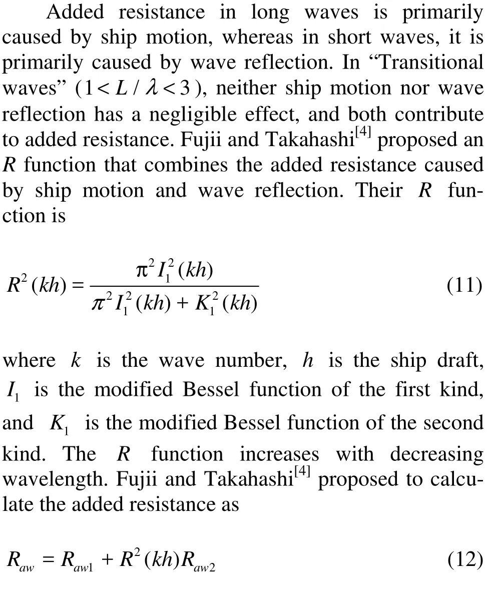
where Raw1is the added resistance caused by ship motion and Raw2is Havelock’s formula for the drift force that is based on wave reflection and uses an empirical correction related to the mean velocity of wave energy transfer. With this R function, the added resistance due to wave reflection is also included for relatively long waves. Therefore, the contributions of ship motion and wave reflection are both included in the total added resistance.

3.2 Combined calculations

Because the added resistance calculated with the radiated energy method or the G & B (Raw1) method is not accurate in short waves, we propose a different use of the R function to gradually reduce the contribution from this term in shorter waves

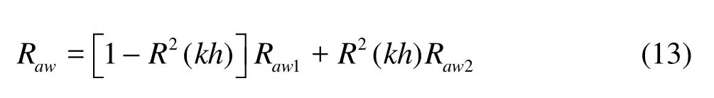
where Raw1is the added resistance calculated using one of the two methods that is valid for long waves (see Subsection 2.1-2.2) and Raw2is the added resistance calculated using the asymptotic formula (see Subsection 2.3). R is given by Eq.(11), which indicates that the contribution of wave reflection to added resistance increases with decreasing wavelength.

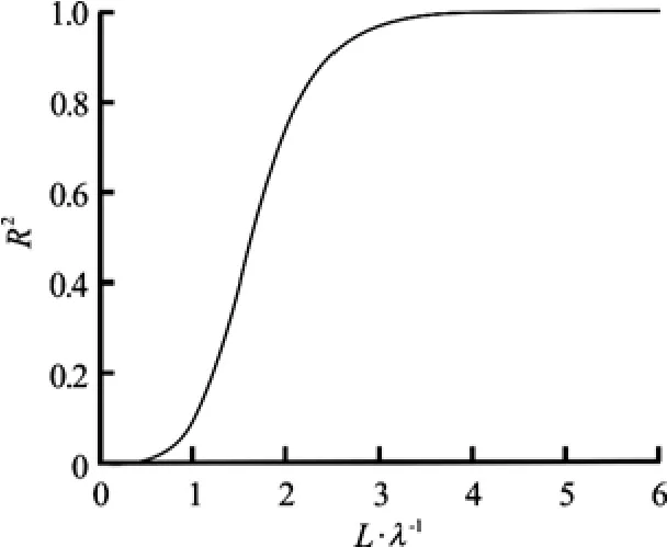
Fig.9 R function vs. L/λ

This trend for KVLCC2 is shown in Fig.9, where the R function increases along the abscissaL/λ. The value of the R function reaches 0.968 at L/ λ= 3, which indicates that ship motion is negligible in short waves, whereas wave reflection can be ignored at L/λ=1, where the value of R reaches 0.086.

This method is consistent with Fuji and Takahashi’s method regarding the transition from long waves to short waves. The difference is that Fuji and Takahashi utilized this method for the different components of total added resistance, whereas this implementation focuses on combining the benefits of different theoretical calculations.

The range of wavelengths used in this experiment is 1.090 ＜ L/λ ＜ 5.526, which includes the most important part of the transition region of R function.

4. Experimental and theoretical results

In this section, the experimental results for the added resistance at different Froude numbers and wavelengths are used to validate the combined calculations discussed above. In addition, the frictional resistance on the friction plate is investigated. The frictional coefficient in calm water and in waves is measured in the experiment, and the results are compared with those from a CFD calculation with Fluent.

4.1 Added resistance

Comparisons of the results of the combined calculations and the experiment for different wave-lengths and Froude numbers are given first.“Exp._total” represents the added resistance coefficient of the whole body, “Exp._fore” represents that of the fore-segment, and “Exp._aft” represents that of the aft-segment.

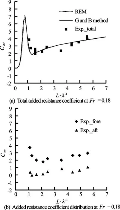
Fig.10 Added resistance at Fr=0.18

Figure 10 shows the added resistance on the whole model and on each segment at Fr =0.18. The total added resistance from experiment is in good agreement with the combined calculations. Figure 10(b) shows that the added resistance is primarily concentrated at the fore-segment, whereas the added resistance at the aft segment is small.

In Fig.10(a), there are four experimental points at L /λ = 5.526, which corresponds to the shortest wave with the lowest wave height, H =0.03m , where added resistance is very difficult to measure accurately. Four runs were performed to increase the accuracy. The added resistance coefficient for each run is Caw=4.270, 4.259, 4.239, and 3.980, which shows that the maximum deviation is only 4.944%.

In Fig.10(a), there are two different experimental points at both L /λ = 4.368 and L/λ = 1.571, which represent the typical regions for short waves and relatively long waves, respectively. These two points represent the added resistance coefficients at two different wave heights and are used to study the effect of wave amplitude on the added resistance. At L/λ = 4.368, two wave heights of H =0.03m and H =0.05 m are chosen. The results are Caw=3.176 at H =0.03m and Caw=3.357at H =0.05 m. At L /λ = 1.571, two runs are performed at wave heights of H =0.03m and H =0.15 m. The added resistance coefficients are Caw=1.980 and 2.599 at H =0.03m and Caw=2.442and 2.263 at H= 0.15 m. The results show that the dimensionless added resistance is nearly independent of the wave amplitude, which confirms that the added resistance for short waves is proportional to the square of the wave amplitude. The scatter in the results at H= 0.03m may be due to the uncertainty in the measured force and wave amplitude.

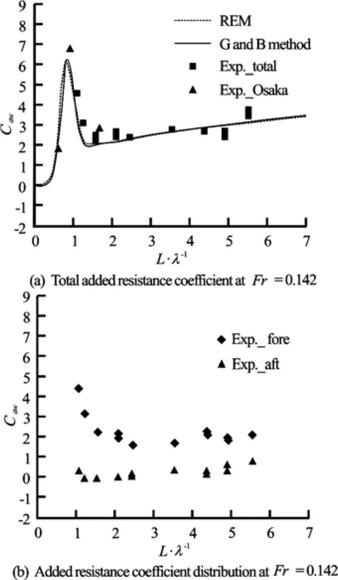
Fig.11 Added resistance at Fr=0.142

Figure 11 shows the added resistance on the whole model and on each segment at Fr =0.142, which is the design speed. The results generally show good agreement between the calculated and the measured total added resistance coefficient.

In Fig.11(a), there are two points at L/λ= 5.526 for two runs. The added resistance coefficients are Caw=3.780 and Caw=3.454, the deviation of which is 4.506%.

The effect of wave amplitude on the added resistance is also studied at L /λ = 1.571 and L/λ= 4.368. Figure 11(a) shows that the added resistance coefficients are very similar for the two waves with the same wavelength and different wave heights,which clearly supports the conclusion that the added resistance coefficient is independent of wave amplitude.

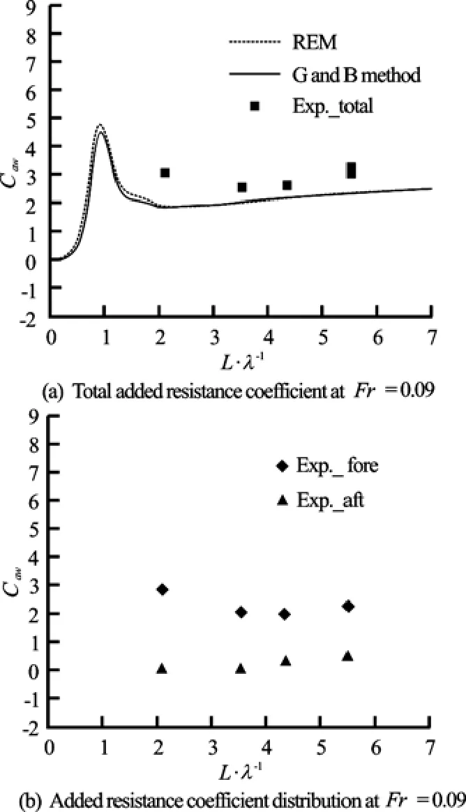
Fig.12 Added resistance at Fr=0.09

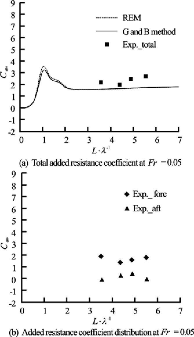
Fig.13 Added resistance at Fr=0.05

Figure 12 shows the added resistance on the whole model and on each segment at Fr =0.09. At this Froude number, the combined calculations underpredict the total added resistance. Similar to the previous case, three runs were performed at L/λ= 5.526, and the added resistance coefficients are Caw=3.087, 3.176, and 3.281, with a maximum deviation of only 2.965%.

Figure 13 shows the added resistance on the whole model and on each segment at Fr =0.05. In short waves, the combined calculations under-predict the total added resistance, similar to the results at Fr =0.09.

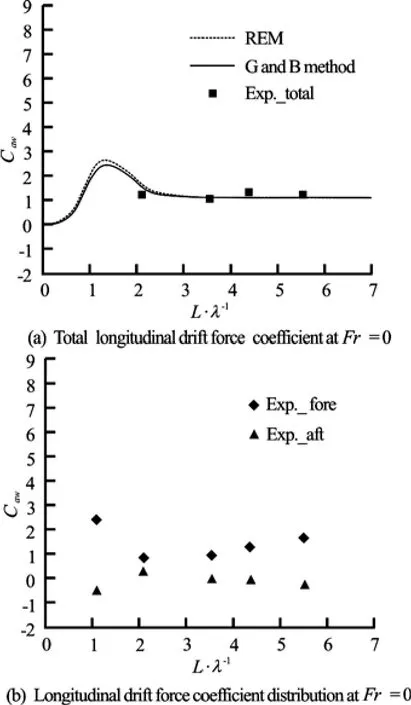
Fig.14 Longitudinal drift force coefficient at Fr=0

Figure 14 shows the longitudinal drift force on the whole model and on each segment at Fr=0. Figure 14(a) shows good agreement between the combined calculations and the experimental results. Actually, at Fr=0, the experiment should ideally be performed in an ocean basin, because waves reflected from the tank wall will affect the incoming wave. However, it is performed in the towing tank for this experiment. To prevent the reflected waves from having an effect, the time window must be very short, especially for the relatively long waves.

4.2 Added frictional resistance

Added resistance is composed of both frictional resistance and pressure resistance. The pressure resistance on the friction plate is zero, the resistance onthis plate only includes frictional resistance. To study the effect of waves on frictional resistance, the frictional resistance on the friction plate (see Fig.3) is investigated. The frictional coefficient Cfmeasured in the experiment is compared with CFD results.

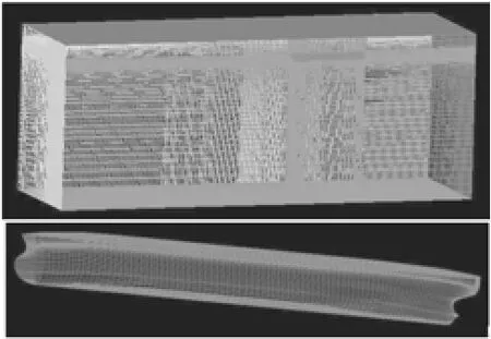
Fig.15 Mesh for CFD calculation

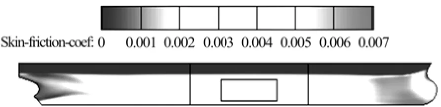
Fig.16 Distribution of the local frictional coefficient

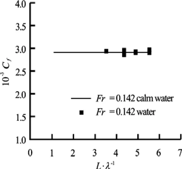
Fig.17 Frictional coefficient of the friction plate in calm water and in waves

4.2.1 Frictional coefficient from CFD

A CFD computation for the ship in calm water is performed at Fr =0.142 using Fluent. The computational domain is ?3 .0 L＜ x ＜ 2.5L , ?0 .01L ＜ y ＜1.5L and ?1 .6 L＜ z ＜ 0.2L , where the symmetry condition is adopted at y=0, and the free surface lies at z=0. The ship’s stern is located at x=0, and the bow is located at x=L. A grid convergence study of ship resistance with respect to the number of nodes is performed, and the results show that a hexahedral mesh with 1 989 559 elements (shown in Fig.15) provides sufficient grid resolution. SST k?ω turbulent model is adopted for the numerical simulation, and Implicit VOF is utilized to capture the free surface. For details, refer to Guo and Steen[15]. A wall function is used to model the flow around the hull, andy+at the wall-adjacent cell is kept in the range of 45-90 except in a limited area close to the stern. It has been demonstrated that a wall function with suitable values of+y can give a very reasonable result.

The average local frictional coefficient of the plate is 0.00303, which is consistent with the experimental result (see Fig.17). The frictional resistance distribution over the entire hull is shown in Fig.16. The CFD results show that the frictional coefficient at the friction plate is almost the same as that at the midsegment.

4.2.2 Frictional coefficient by experiment

The frictional coefficient on the friction plate is calculated as

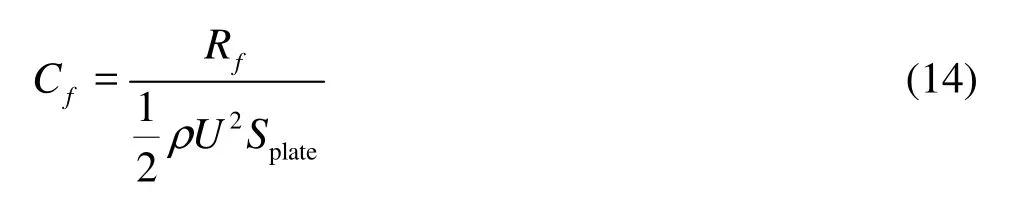
where Rfis the frictional resistance measured by the friction plate, U is model velocity, and Splateis the area of the friction plate. Figure 17 shows the frictional coefficient in calm water and in waves at Fr =0.142.

The added frictional resistance due to waves is very small in very short waves, which indicates that very short waves have a small effect on the frictional resistance of the friction plate. The frictional coefficients in relatively long waves are not given because the frictional plate is partly out of water in this wavelength region as a result of relative wave motion.

5. Uncertainty analyses

The uncertainty in the experimental measurements is provided for the validation of the numerical calculations. The methodology and procedures for experimental uncertainty that are recommended by the ITTC (2002)[16]are followed here. The error is divided into bias and precision errors, which can be estimated using a bias limit and a precision limit at 95% confidence level. Bias errors are systematic errors that can be estimated by evaluating the elemental error sources for individual variables, and precision limit is “scatter”in the results that can be calculated by performing multiple tests with the same test conditions.

5.1 Bias limit

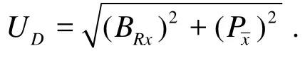
The procedure described by Longo and Stern[17]is followed here to estimate the bias limit. The bias limit of the resistance BRxis composed of three uncorrelated elemental limits (BRx1, BRx2, BRx3) . It is calculated as BRx=. The data are given in Table 3.

The error in the calibration for the resistance transducer BRx1arises from the error in the calibra-tion weight. BRx2is due to misalignment or the difference between the calibration and the test conditions for the force transducer. BRx3arises from the scatter of the calibration data in relation to a linear least-squares regression fit curve. The terms in Table 3 are the total resistance Rt, resistance at the fore segment Rfore, resistance at the aft segment Raftand frictional resistance of the friction plate Fplate.

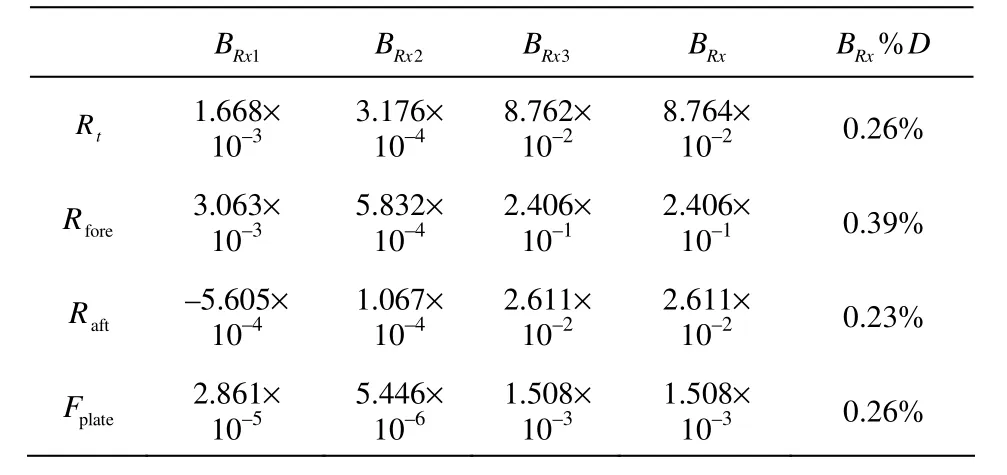
Table 3 Bias error for the force transducer

5.2 Precision limit

The precision error provides a quantitative measure of the reliability of the measured resistance and shows that the use of multiple time windows can improve the results. In this experiment, several repetitions were performed to determine the calm water resistance.

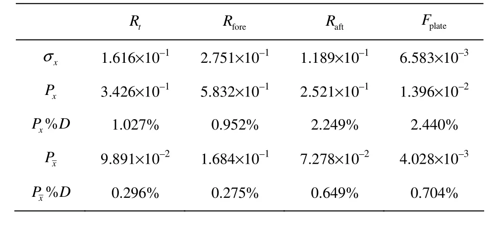
Table 4 Precision error for 1 time window

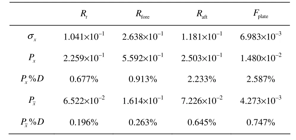
Table 5 Precision error for 1 000 time windows

Sixteen runs were performed in calm water, and the precision error analysis is shown in Table 4 and Table 5.

The confidence interval is set at 95%, and a precision limit is found for a sample (Px) and for the mean of all samples (Px). In addition, the standard deviation σx, Px%D and Px%D are given. D is the mean measured force. Table 4 shows the precision error analysis of the force from one time window, and Table 5 shows the results found by averaging 1 000 time windows.

A comparison of the results shows that using multiple time windows significantly reduces the precision error in the total resistance, although there is no significant reduction in the other force components. This result could be expected because the analysis using multiple time windows was implemented to eliminate the effect of the slowly varying component of the total resistance measurement, and there is little or no slowly varying component in the other resistances. The uncertainty in the force at each segment is larger than that in the total resistance. A possible explanation for this finding is that the force transducer on each segment moves with the ship model, and thus, more disturbances are introduced. Additionally, the springs that are required to transfer vertical forces and the sealing that is required to make the cuts between the sections watertight might increase the uncertainty in the component resistance measurements.

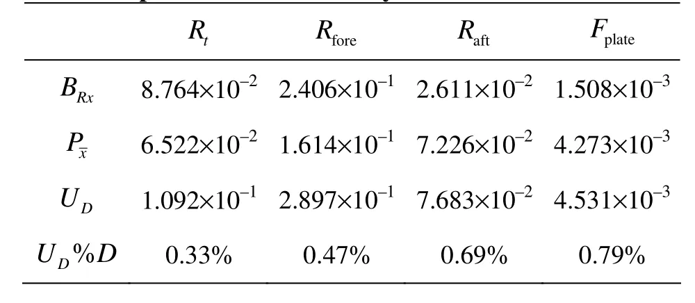
Table 6 Experimental uncertainty

5.3 Uncertainty of experimental data

Due to financial concerns, an uncertainty analysis for the added resistance measurement is not provided here. Repeated tests with certain waves, such as L /λ = 5.526 and L /λ = 4.896, are utilized to check the repeatability of the experimental results, but these tests are insufficient as a formal uncertainty analysis. In addition, the uncertainty in the added resistance should be smaller than that in the calm water resistance. The precision error in the calm water test includes the error due to the residual waves from the last run because calm water cannot be strictly ensured after each run due to a limited time between runs (approximately 30 min). However, this error does notnoticeably affect the final result of the added resistance because the wave resistance measurement is performed immediately after the calm water measurement, and this error is cancelled by subtracting the mean resistance in calm water from that in waves. Figures 10(a)-12(a) show good repeatability for the added resistance measurements.

6. Conclusions

Experiments to determine the added resistance in short waves were performed, and the results are analyzed and compared using two types of combined calculations. The conclusions include the following points:

(1) A model test of added resistance in short waves is very difficult due to the small wave amplitude and the measured force. A detailed wave calibration should be carefully performed before the experiment. To achieve more accurate results, a new data processing method is proposed to effectively eliminate the effect of low-frequency noise in the measured force.

(2) The “REM” and “G & B” methods cannot satisfactorily predict the added resistance in short waves, but they can predict the added resistance of KVLCC2 in long waves. The asymptotic formula gives good predictions for the KVLCC2 in short waves. However, the application region of the asymptotic formula is limited, but by combining “REM”and “G & B” with an R function, the added resistance can be predicted well over the entire wavelength region.

(3) The added resistance calculated using the combined method is slightly under-estimated at low Froude numbers. For higher Froude numbers and zero speed, the added resistance computational results match the experimental results very well.

(4) A unique characteristic of this experiment is that the model is divided into three segments to study the distribution of the added resistance. The experimental results show that the added resistance is concentrated at the fore-segment and that it is small at the aft-segment. Thus, an optimization of the bow shape could effectively reduce the added resistance. In the mid-segment, the increase of frictional resistance on the friction plate due to short waves is very small.

(5) The dimensionless added resistance coefficient measured by experiment is fairly independent of wave amplitude, which confirms that the added resistance for short waves is roughly proportional to the square of the wave amplitude.

In future experiments, the effect of the ship geometry on the added resistance will be studied.

Acknowledgements

The author acknowledges the discussions with Senior Research Engineer Dariusz Fathi and the experimental assistance from ?rjan Selvik in MARINTEK. This work is part of the research project SeaPro, which is sponsored by Rolls-Royce Marine and the Research Council of Norway.

[1] FALTINSEN O. M. Hydrodynamics of high-speed marine vehicles[M]. Cambridge, UK: Cambridge University Press, 2006, 238-240.

[2] ITTC. Testing and extrapolation methods, propulsion, performance, prediction powering margins. ITTC-recommended procedure and guidelines[C]. Proceeding of 23rd International Towing Tank Conference (ITTC). Venice, Italy, 2002, 1-14.

[3] IMO. Prevention of air pollution from ships[C]. Marine Environment Protection Committee, International Maritime Organization (IMO). Oslo, Norway, 2008, 1-4.

[4] FUJII H., TAKAHASHI T. Experimental study on the resistance increase of a ship in regular oblique waves[C]. Proceeding of 14th International Towing Tank Conference. 1975, 351-360.

[5] FALTINSEN O. M., MINSAAS K. J. and LIAPIS N. et al. Prediction of resistance and propulsion of a ship in a seaway[C]. Proceeding of 13th Symposium on Naval Hydrodynamics. Tokyo, Janpan, 1980, 505-529.

[6] GUO B. J., STEEN S. Experiment on added resistance in short waves[C]. Proceeding of 28th Symposium on Naval Hydrodynamics. Pasadena, USA, 2010.

[7] STEEN S., FALTINSEN O. M. Added resistance of a ship moving in small sea states[C]. Practical Design of Ships and Mobile Units. Hague, The Netherlands, 1998.

[8] TSUJIMOTO M., KURODA M. and SHIBATA K. et al. Development of a practical calculation method for added resistance in short waves[C]. The 8th Research Presentation Meeting of National Maritime Research Institute. Tokyo, Japan, 2008, 1-9.

[9] KIM W. J., VAN S. H. and KIM D. H. Measurement of flows around modern commercial ship models[J]. Journal of Experiments in Fluids, 2001, 31(5): 567-578.

[10] LEE S. J., KIM H. R. and KIM W. J. et al. Wind tunnel tests on flow characteristics of the kriso 3600 TEU containership and 300K VLCC double-deck ship models[J]. Journal of Ship Research, 2003, 47(1): 24-38.

[11] LARSSON L., STERN F. and VISONNEAU M. Gothenburg 2010 a workshop on numerical ship hydrodynamics[C]. Proceedings of Gothenburg 2010 Workshop on Numerical Ship Hydrodynamics. Gothenburg, Sweden, 2010.

[12] SIMMAN. MOERI Tanker KVLCC2[C]. Workshop on Verification and Validation of Ship Manoeuvering Simulation Methods(SIMMAN 2008). Copenhagen, Denmark, 2008.

[13] GUO B. J., STEEN S. Added resistance of a VLCC in short waves[C]. Proceeding of 29th International Conference on Ocean, Offshore and Arctic Engineering (OMAE 2010). Shanghai, 2010.

[14] STANSBERG C. T. Wave field homogeneity in MARINTEK’s towing tank I+III[M]. Trondheim, Norway: MARINTEK, 2004, 1-34.

[15] GUO B. J., STEEN S. Computational study on ship resistance and flow field of KVLCC2[C]. Proceedings of Gothenburg 2010 Workshop on Numerical Ship Hydrodynamics. Gothenburg, Sweden, 2010, 585-593.

[16] ITTC. Resistance uncertainty analysis, example for resistance test[C]. Proceeding of 23rd International Towing Tank Conference (ITTC). Venice, Italy, 2002, 1-18.

[17] LONGGO J., STERN F. Uncertainty assessment for towing tank tests with example for surface combatant dtmb model 5415[J]. Journal of Ship research, 2005, 49(1): 55-68.

10.1016/S1001-6058(10)60168-0

* Biography: GUO Bing-jie (1982-), Female, Ph. D. Candidate

STEEN Sverre, E-mail: sverre.steen@ntnu.no