
PROPERTIES OF NATURAL CAVITATION FLOWS AROUND A 2-D WEDGE IN SHALLOW WATER*
2011-05-08 05:54CHENXin
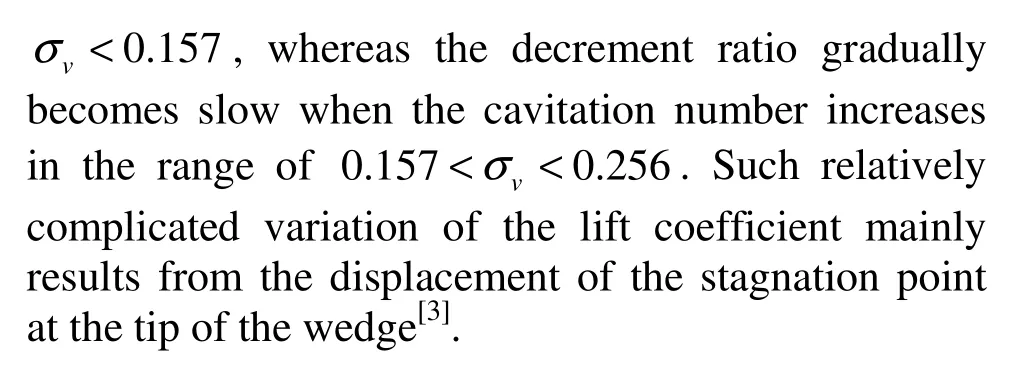
水動力學研究與進展 B輯 2011年6期
CHEN Xin
Department of Engineering Mechanics, Shanghai Jiao Tong University, Shanghai 200240, China, E-mail: xinchen@sjtu.edu.cn
LU Chuan-jing
Department of Engineering Mechanics and State Key Laboratory of Ocean Engineering, Shanghai Jiao Tong University, Shanghai 200240, China
LI Jie, CHEN Ying
Department of Engineering Mechanics, Shanghai Jiao Tong University, Shanghai 200240, China
PROPERTIES OF NATURAL CAVITATION FLOWS AROUND A 2-D WEDGE IN SHALLOW WATER*
CHEN Xin
Department of Engineering Mechanics, Shanghai Jiao Tong University, Shanghai 200240, China, E-mail: xinchen@sjtu.edu.cn
LU Chuan-jing
Department of Engineering Mechanics and State Key Laboratory of Ocean Engineering, Shanghai Jiao Tong University, Shanghai 200240, China
LI Jie, CHEN Ying
Department of Engineering Mechanics, Shanghai Jiao Tong University, Shanghai 200240, China
(Received December 26, 2010, Revised July 10, 2011)
When a body navigates with cavity in shallow water, both flexible free surface and rigid bottom wall will produce great influences on the cavity shape and hydrodynamic performances, and further affect the motion attitude and stability of the body. In the present work, characteristics of the natural cavitating flow around a 2-D symmetrical wedge in shallow water were investigated and the influences of two type boundaries on the flow pattern were analyzed. The Volume Of Fluid (VOF) multiphase flow method which is suitable for free surface problems was utilized, coupled with a natural cavitation model to deal with the mass-transfer process between liquid and vapor phases. Within the range of the cavitation number for computation (0.07-1.81), the cavity configurations would be divided into three types, viz., stable type, transition type and wake-vortex type. In this article, the shapes of the free surface and the cavity surface, and the hydrodynamic performance of the wedge were discussed under the conditions of relatively small cavitation number (<0.256). The present numerical cavity lengths generally accord with experimental data. When the cavitation number was decreased, the cavity was found to become longer and thicker, and the scope of the deformation of the free surface also gradually extends. The free surface and the upper cavity surface correspond fairly to their shapes. However, the lower side of the cavity surface was rather leveled due to the influence of wall boundary. The lift and drag coefficients of this 2-D wedge basically keep linear relations with the natural cavitation number smaller than 0.157, whereas direct proportion for drag and inverse proportion for lift.
shallow water, natural cavitation, boundary effect, multiphase flow
Introduction
When a high-speed underwater vehicle encapsulated in cavity navigates in shallow water, like offshore area, both the flexible free surface and the rigid water bottom will produce obvious influence on the cavity shape and the hydrodynamic performance of the vehicle. In such case, the so called “boundary effect” will make the flow blocked and affect the motion attitude and stability of the vehicle.
Regarding the boundary effect problems caused by solid wall, many researches have been conducted so far in the world through the approaches of theoretical analysis, numerical simulation and experimental investigation. Zhou et al.[1]numerically studied the difference between water tunnel experiments and infinite flow field, including the influence of the route loss and the blocking effect in a water tunnel. They claimed that the wall of the water tunnel should be smoothed to reduce not only the blocking effect but also the pressure drop as far as possible. Chen et al.[2]utilized the multiphase model based on the RANS equations to numerically analyze the wall effect on ventilated cavitating flows around a kind of under-water vehicles with a disk cavitator in a closed water tunnel.
In addition, some other researches concerning about the free surface effect on cavitating flows also have been performed. Franc and Michel[3]calculated the relation of the ratio of lift coefficient to attack angle with the immersion depth of a cavitated hydrofoil beneath water surface, on the basis of the linear theory for an infinite unbounded cavity (with cavitation number of zero). It was suggested from the numerical results that the slope of the relation curve approaches to be constant when the immersion depth is small enough or tends towards infinity.
However, boundary effects on cavitating flows when a rigid wall and free surface coexist have not been widely investigated yet so far. Bal et al.[4]extended the capability of boundary element method[5-7]to the computation of cavitating flows around hydrofoils in a numerical wave tank, with wall effect and free-surface effect simultaneously taken into account. Amromin[8]employed a corrected Riaboushinsky closure model for ideal fluid to numerically analyze the shallow-water effect on supercavitating flows. The computational results indicated that when the same cavity length is reached, the cavitation number under the coaction of a rigid wall and a free surface is greater than that of axisymmetric flow, and the cross section of cavity has some 3-D deformation.
Former literatures regarding the shallow water effect on cavitating flow were mostly limited in the area of potential flow theory, which has difficulty in describing the subtle structure inside the cavity and near the wake. Furthermore, the viscous effect is impossible to be considered in the framework of potential flow. Consequently, in the present work, numerical simulation based on the viscous multiphase flow model[9-11]is carried out to study the boundary effect problem in the natural cavitating flow around a twodimensional wedge in shallow water.
1. Mathematical model and numerical method
In the present work, the VOF multiphase flow model based on the isotropic hypothesis for fluid and the Reynolds Averaged Navier-Stokes (RANS) equations were employed. The mixture medium composed of liquid, vapor and air is regarded as a kind of singlephase fluid with variable density. Each component phase shares the same physical fields, viz., pressure, velocity and so on. The gravity effect of liquid was considered and the compressibility of gas was neglected. The volume fractions of air, vapor, and liquid phases, denoted asaα,vα andlα respectively, are introduced to obtain a set of governing equations describing the multiphase flow of air, vapor, and liquid phases.
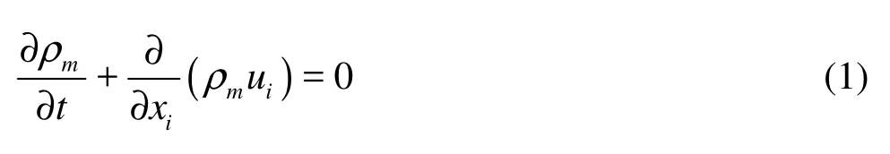
The continuity equation for the mixture is as follows
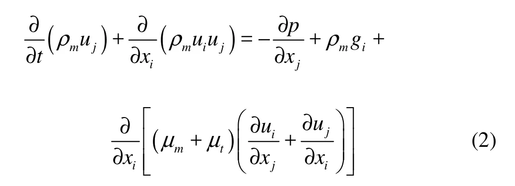
The momentum theorem for the mixture holds as
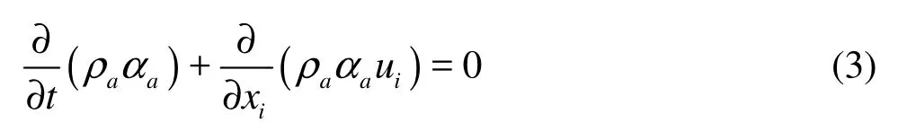
The air phase should keep continuous
The vapor phase should also satisfy continuity during phase-transition process
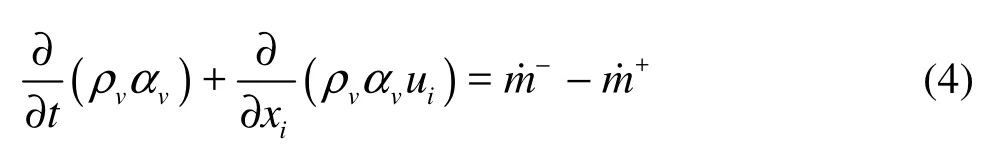
where ρ is the density, t the time, uieach velocity component, p the local pressure, the subscripts m, a, v and l respectively indicate the mixture, air, vapor and liquid phases, i and j indicate the Cartesian coordinates which can be 1, 2 or 3.
A compatible equation holds for the three phases

Additionally, two individual transportation equations were employed to describe the phase-transition process[12]given as Eq.(4) between the vapor phase and the liquid phase.
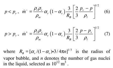
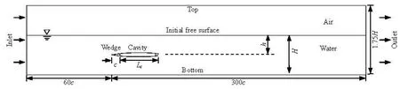
Fig.1 Computational domain and boundary specification
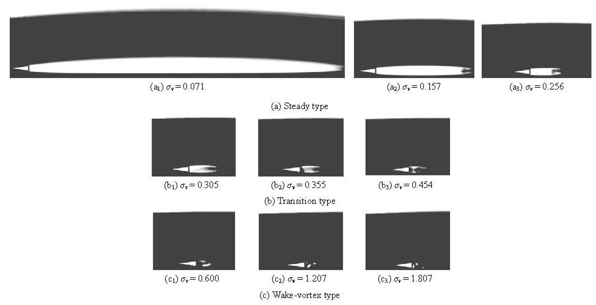
Fig.2 Three types of cavity patterns
The density and viscosity of the mixture were calculated as the weighted average of the volume fraction of each phase:
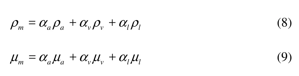
Moreover, the reliable k?ε turbulence model[13]together with the standard wall function[14]is used to calculate the turbulence viscosity,tμ, to make the governing equations closed.
The finite volume method was utilized to discretize the integral governing equations, and the HRIC high-order convection scheme[15]was employed to capture the free surface. In the equations, the temporal term was discretized with a firs-order implicit scheme, and a second-order upwind scheme was adopted for both the pressure term and the convection term. The convection term in turbulence model equation was approximated with a first-order upwind scheme especially. A SIMPLE typed algorithm[16]was employed to consider the pressure-velocity-density coupling solving process. The ultimately linearized algebra equation was solved with the Gauss-Seidel iteration method[17]and accelerated using algebraic multigrid method. In computation, a time step of 10–4s was selected to divide the total time span of 0.15 s-0.2 s, and the number of iteration in each time step was set to be 50.
2. Computational domain and boundary conditions
The 2-D computational domain and boundary conditions are illustrated in Fig.1, where the length and the bottom width of the symmetric wedge are respectively c =0.06 m and D=0.017 m (R=0.5D). The origin of the coordinate system is located at the tip of the wedge, which has an immersion depth of h =0.14 m in the water with a free surface of H= 0.28 m high from the water bottom. The external boundary of the computational domain is 1.75H from the bottom. The positive directions of x and y axes point rightward and upward respectively. The upstream boundary and the downstream boundary are respectively 60c and 300c away from the origin.The domain was divided into multi-block structured mesh with 100 800 cells.
The physical boundaries are assigned with suitable conditions. The upstream boundary and the upper external boundary were disposed with constant velocity (u1=0 m/s for y>h, or else u1= 10 m/s, u2=0 m/s). The downstream boundary was specified with fixed static pressure (poutlet= P0for y>h, or else poutlet= P0?ρlgy), which was used to adjust the cavitation number. The surface of the wedge and the bottom boundary were given as the noslip wall condition.
3. Results and discussion
In this section, the influence of boundary effects on several aspects, including cavity pattern, free surface shape and hydrodynamics of the wedge, are discussed as follows.
3.1 Cavity pattern
Figure 2 presents the computed cavity patterns with the free surface at some specific values of cavitation number, which is defined as σv=(P∞?pv)/ 0.5ρV2. The cavity outline is defined as the interface
l∞where the iso-surface of αv=0.5 locates, in which pvindicates the saturated vapor pressure of water at specific temperature, and P∞and V∞denote respectively the environment pressure and free-stream velocity.
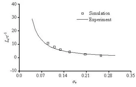
Fig.3 Relation betweenvσ (<0.256) and Lc
It seems obvious that cavity size would shrink if cavitation number increases. The cavity can generally be divided into the three types as follows:
(1) Steady type.vσ is approximately in the range of 0.07-0.3. The cavity presents the state of supercavity which is nearly full of pure vapor. The cavity profiles keep stable except for the tiny oscillation near the cavity tail.
(2) Transition type.vσ is approximately in the range of 0.3-0.5. The cavity presents the state of cloudy mixture composed of vapor and liquid, which is produced by the strong reentrant jet generated from the tail of the cavity. The cavity can roughly keep relatively clear outline.
(3) Wake-vortex type. σvis approximately in the range of 0.5-1.81. The cavity presents the state of vortex cavitation, which occurs in the shedding vortex of the wake and exhibits an evident periodicity.
3.2 Shapes of free surface and cavity interface
Because the cavity shapes of the transition type and wake-vortex type are not stable enough to be analyzed quantitatively, only the steady type of cavity is selected to be discussed in this section.
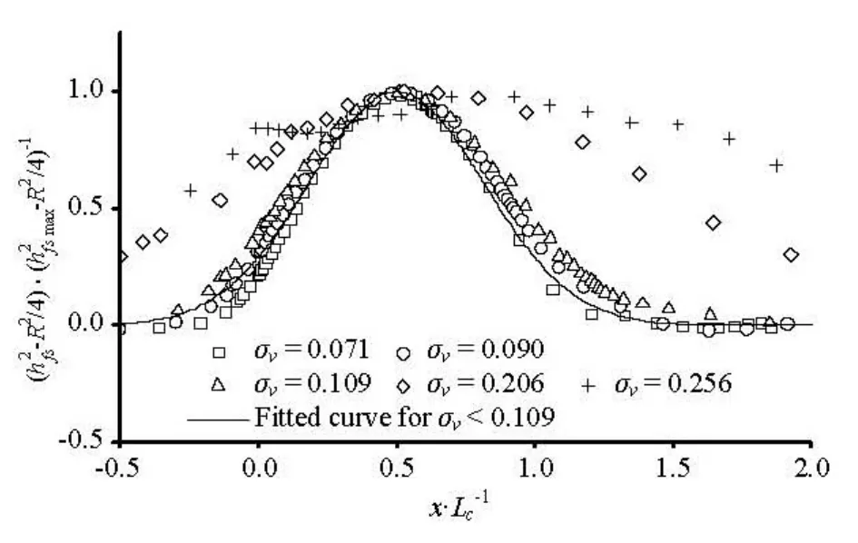
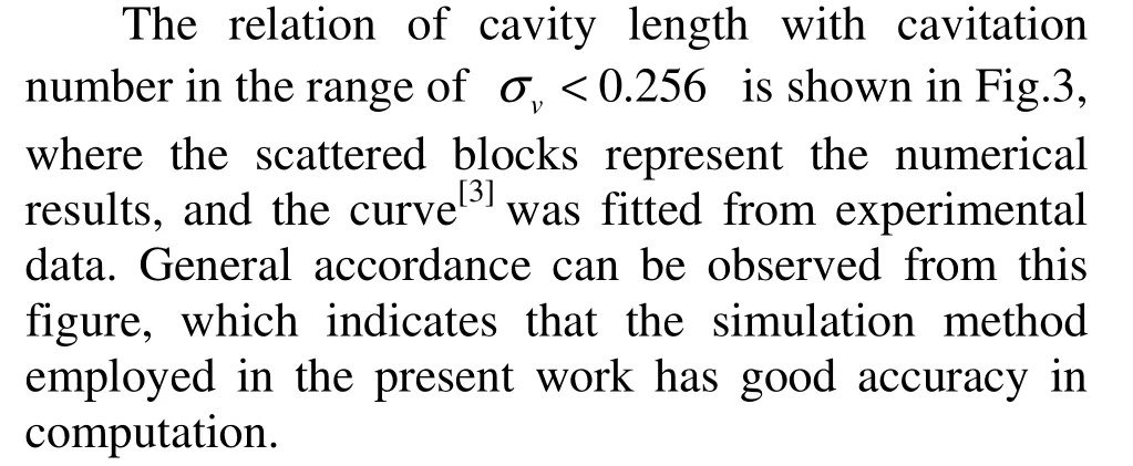
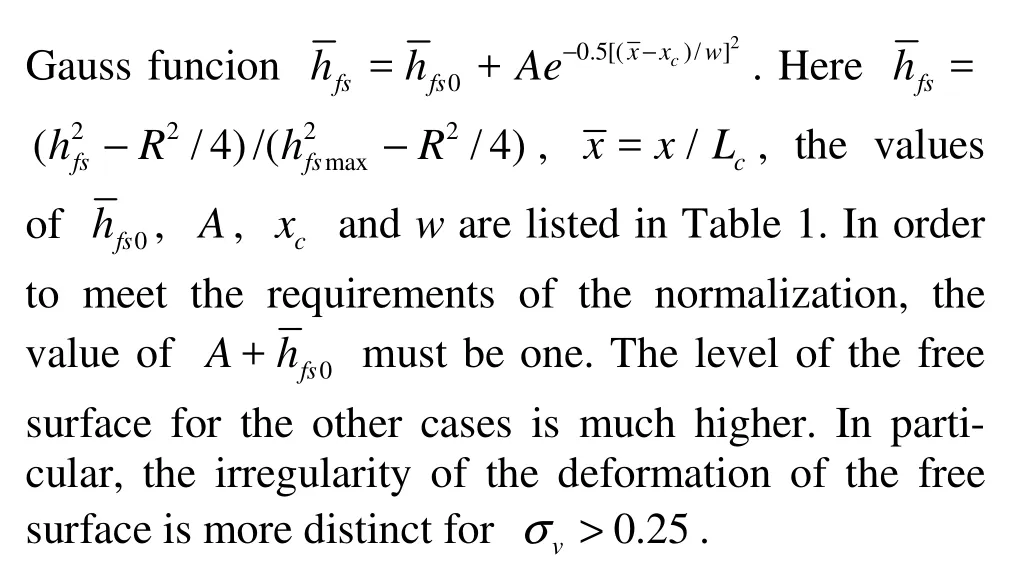
Fig.4 Universal profiles of free surface for various values of vσ (<0.256)
The height differences hfsbetween the free surfaces at the conditions of after deformation and of at still status, were normalized as to the maximal height difference hfsmax, to obtain a universal free surface in small cavitation number condition as shown in Fig.4, where the free surfaces are defined as the contour of αa=0.5.
Table 1 Parameters in the Gauss function fitted for the profile of free surface
It can be observed from the figure that the shapes of the free surfaces in the cases for σv< 0.109 are close to each other, approaching the curve of the
The influence of the free surface is quite different from that of the solid wall on the shape of the cavity. Thus, the upper and lower surface of the cavity must be discussed respectively.
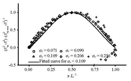
Fig.5 Universal profiles of the upper surface of cavity at variousvσ (<0.256)
Figure 5 presents the profiles of the upper surface of cavity along the axial direction when the cavity width Rupare normalized as to the maximal cavity width Rupmax, where the cavity width is defined as the vertical length from any specific point on cavity surface to the symmetry line of the wedge.
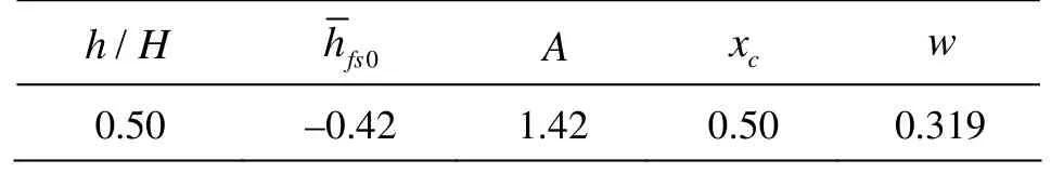
Table 2 Parameters in the Gauss function fitted for the profile of the upper surface of cavity
It is obvious to notice that the upper cavity surfaces present pretty good unity except for some disagreement at the tail of the cavity due to the presence of reentrant jets. In a range of one cavity length, after some simple translations of fitting curve in Fig.4, it is found that the shape of the upper cavity surface basically accords with that of the free surface in the axial extent around the cavity, and approximately looks symmetric right-and-left about the abscissa of x =0.5Lc. Such phenomenon owes to the flexibility of free surface which deforms along with the development of cavity surface. All the parameters for the fitting curves in Fig.5 are listed in Table 2. Strictly speaking, the shape of the cavity’s upper surface is more appropriate to the curve of parabolic function. Here, the curve of Gauss function is adopted just for illustration of the similarity between profiles of the upper cavity surface and those of the free surface.
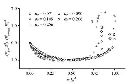
Fig.6 Universal profiles of the lower surface of cavity for various values ofvσ (<0.256)
Additionally, Fig.6 presents the profile of the lower surface of cavity. The lower cavity radiuses Rlowwere normalized as to the maximal lower radius Rlowmax.
The cavity tails at the conditions of σv=0.206 and σv=0.256 also have evident disagreement as in the other cases, which also results from the shedding and concavity of cavity caused by the reentrant jet. As a whole, the lower surface has relatively poorer consistency than the upper surface. In the majority of the cavitating region, the lower surface looks flatter than the upper one. Such result is regarded reasonable due to the existence of the rigid bottom wall, which prevents the lower surface of the cavity from developing in the vertical direction. Since there is a big difference in shapes of the cavity’s lower surface, it is difficult that a universal fitting curve can be given.
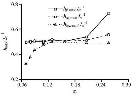
Fig.7 Positions located in the maximum of the level of free surface and the width of cavity surface for various values of vσ
Figure 7 shows the relations between the cavitation number with positions located at the maximum level of the free surface as well as the width of cavity surface.
For σv> 0.2 in the rough, the positions for the maximal width of the upper and lower surface of cavity is close to each other, but the position for the maximal level of the free surface obviously moves backward. When the cavitation number σvis roughly smaller than 0.2, the position located in the maximal level of free surface is close to that in the maximal width of cavity’s upper and lower surfaces, which implies that the profiles of the free surface and the cavity’s surface maintain right-and-left symmetry. However, for σv< 0.1, with the dropping σvthe position for the maximal width of the cavity’s lower surface moves forward, which reveals the up-anddown symmetrically shape of cavity surface is destroyed. From these geometrical results one can see that the influence of the solid wall on the shape of the free surface and cavity interface is much stronger than that of the flexible free surface.
3.3 Hydrodynamic properties
Since the instability of cavity could also induce the hydrodynamic properties to oscillate, we still use the computational cases of cavity of steady type to analyze in this section.
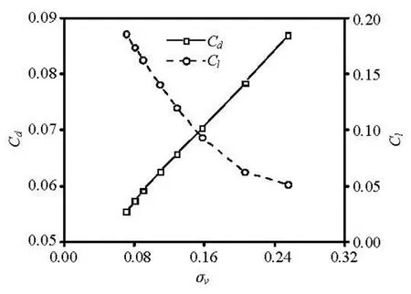
Fig.8 Variation of Cdand Clalong withvσ
Figure 8 presents the relation between cavitation number and the numerical predicted drag and lift coefficients defined respectively as Cd= Fx/0.5ρlV∞2c and Cl= Fy/0.5ρlV∞2c , where Fxand Fyrespectively denote the component of the resultant force acting on the wedge in the x direction and y direction.
It is clearly indicated from the curves that the drag coefficient nearly keeps linear in direct proportion with cavitation number for the steady type of cavity (σv< 0.256). However, the lift coefficient just keeps linear in inverse proportion only in the range of
4. Conclusions
In the present work, cavity patterns and hydrodynamic properties of the natural cavitating flows around a 2-D wedge in shallow water have been numerically investigated using the VOF multiphase flow model based on the RANS equations coupled with a cavitation model. The influence of two types of boundaries on the cavity pattern has been analyzed and compared with experimental results. Some conclusions as follows can be drawn from the above analysis:
(1) In the range of the computational cavitation number in this work (0.07 < σv< 1.81), the cavity pattern can be divided into three types as steady type, transition type and wake-vortex type. The successful prediction of the cavity of wake-vortex type indicates that the viscous multiphase model has evident advantage against the simulation methods in traditional framework of potential flow.
(2) For the steady type of cavity, the computed cavity length basically accords with the corresponding experimental one. Along with the reduction of cavitation number, cavity size increases as well the deformation region of free surface. The free surface generally keeps consistent with the upper surface of cavity in their shapes. However, the lower surface of cavity looks flatter due to the restriction of its development in vertical direction by the effect of rigid water bottom.
(3) Under the condition of σv< 0.157, the lift and drag coefficients of the 2-D wedge both nearly keep linear relation with the cavitation number. Moreover, the drag coefficient presents a direct proportion with cavitation number, but the lift coefficient just behaves on the contrary.
[1] ZHOU Jing-jun, YU Kai-ping and MIN Jing-xin et al. The comparative study of ventilated super cavity shape in water tunnel and infinite flow field[J]. Journal of Hydrodynamics, 2010, 22(5): 689-696.
[2] CHEN Xin, LU Chuan-jing and LI Jie et al. The wall effect on ventilated cavitating flows in closed cavitation tunnels[J]. Journal of Hydrodynamics, 2008, 20(5): 561-566.
[3] FRANC J. P., MICHEL J. M. Fundamentals of cavitation[M]. Dordrecht, The Netherlands: Kluwer Academic Publisher, 2004.
[4] BAL S., KINNAS S. A. A BEM for the prediction of free surface effects on cavitating hydrofoils[J]. Computational Mechanics, 2002, 28(3-4): 260-274.
[5] BAL S., KINNAS S. A. and LEE H. Numerical analysis of 2-D and 3-D cavitating hydrofoils under a free surface[J]. Journal of Ship Research, 2001, 45(1): 34-49.
[6] BAL S. High-speed submerged and surface piercing cavitating hydrofoils, including tandem case[J]. Ocean Engineering, 2007, 34(14-15): 1935-1946.
[7] BAL S., KINNAS S. A. A numerical wave tank model for cavitating hydrofoils[J]. Computational Mechanics, 2003, 32(4-6): 259-268.
[8] AMROMIN E. Analysis of body supercavitation in shallow water[J]. Ocean Engineering, 2007, 34(11-12): 1602-1606.
[9] SINGHAL A. K., ATHAVALE M. M. and LI H. Y. et al. Mathematical basis and validation of the full cavitation model[J]. Journal of Fluids Engineering, 2002, 124(3): 617-624.
[10] CHEN Xin, YAO Yan and LU Chuan-jing et al. Interference of foil-shaped side strut on the natural cavitating flows over submerged vehicle in water tunnel[J]. Journal of Hydrodynamics, 2011, 23(5): 554-561.
[11] CAO Da-min, XU Xu. Numerical simulation of cavitation flow field for under water projectile[J]. Journal of Beijing University of Aeronautics and Astronautics, 2008, 34(10): 1191-1194,1199(in Chinese).
[12] SCHNERR G. H., SAUER J. Physical and numerical modeling of unsteady cavitation dynamics[C]. Fourth International Conference on Multiphase Flow. Louisiana, New Orleans, USA, 2001.
[13] SHIH T. H., LIOU W. W. and SHABBIR A. et al. A new k?ε eddy-viscosity model for high Reynolds number turbulent flows-model development and validation[J]. Computers Fluids, 1995, 24(3): 227-238.
[14] NG E. Y. K., TAN H. Y. and LIM H. N. et al. Nearwall function for turbulence closure models[J]. Computational Mechanics, 2002, 29(2): 178-181.
[15] WALTERS D. K., WOLGEMUTH N. M. An improved high-resolution discretization scheme for volume-offluid CFD simulations[C]. Proceedings of the 5th Joint ASME/JSME Fluids Engineering Summer Conference. San Diego, USA, 2007.
[16] YANG Guo-gang, DING Xin-wei and BI Ming-shu et al. Improved SIMPLE algorithm used in numerical simulation of flammable gas cloud deflagration[J]. Journal of Dalian University of Technology, 2004, 44(6): 789-792(in Chinese).
[17] CHENG Guang-hui, HUANG Ting-zhu and CHENG Xiao-yu. Preconditioned gauss-seidel type iterative method for solving linear systems[J]. Applied Mathematics and Mechanics (English Edition), 2006, 27(9): 1275-1279.
10.1016/S1001-6058(10)60170-9
* Project supported by the National Natural Science Foundation of China (Grant Nos. 11002089, 10832007) the Shanghai Leading Academic Discipline Project (Grant No. B206).
Biography: CHEN Xin (1976-), Male, Ph. D., Lecturer

- 水動力學研究與進展 B輯的其它文章
- LATTICE BOLTZMANN METHOD SIMULATIONS FOR MULTIPHASE FLUIDS WITH REDICH-KWONG EQUATION OF STATE*
- DYNAMIC ANALYSIS OF FLUID–STRUCTURE INTERACTION OF ENDOLYMPH AND CUPULA IN THE LATERAL SEMICIRCULAR CANAL OF INNER EAR*
- SIMULATIONS OF FLOW INDUCED CORROSION IN API DRILLPIPE CONNECTOR*
- NUMERICAL SIMULATION OF FLOW OVER TWO SIDE-BY-SIDE CIRCULAR CYLINDERS*
- NUMERICAL STUDY OF HYDRODYNAMICS OF MULTIPLE TANDEM JETS IN CROSS FLOW*
- EXPERIMENTAL STUDY ON SEDIMENT RESUSPENSION IN TAIHU LAKE UNDER DIFFERENT HYDRODYNAMIC DISTURBANCES*