EXPERIMENTAL AND NUMERICAL STUDIES OF AERODYNAMIC PERFORMANCE OF TRUCKS*

QI Xiao-ni, LIU Yong-qi

School of Transportation and Vehicle Engineering, Shandong University of Technology, Zibo 255049, China, E-mail: qixiaoni@sjtu.org

DU Guang-sheng

School of Energy and Power Engineering, Shandong University, Jinan 255061, China

EXPERIMENTAL AND NUMERICAL STUDIES OF AERODYNAMIC PERFORMANCE OF TRUCKS*

QI Xiao-ni, LIU Yong-qi

School of Transportation and Vehicle Engineering, Shandong University of Technology, Zibo 255049, China, E-mail: qixiaoni@sjtu.org

DU Guang-sheng

School of Energy and Power Engineering, Shandong University, Jinan 255061, China

(Received April 7, 2011, Revised July 18, 2011)

This article studies the truck-induced airflow. The results of numerical investigations are used to assess the effectiveness of the installed hash symbol (#) shaped fence on the truck. The Reynolds-averaged Navier-Stokes equations are solved using the finite volume method. The computed distributions of the pressure and the air velocity as well as the computed aerodynamic drag coefficients reveal the effects of a fence on the aerodynamic performance of the truck. It is shown that the hash symbol shaped fence plays its role due to its aerodynamic characteristics, better than those of the original model. For various gaps, the optimal position and height of fences are discussed in the article.The experiments in a low speed wind tunnel provide the edidence for validation.

truck, numerical simulation, wind tunnel, fence

Introduction

Two thirds of the goods in China are transported by trucks. 50%-70% of the truck’s power (at 70 km/h-100 km/h speed) is consumed in overcoming the aerodynamic resistance. This fact suggests that even 1% reduction in the aerodynamic drag would amount to a significant saving in the fuel cost[1,2]. As the traveling speed increases, the aerodynamic resistance increases in a direct proportion to the square of the speed, and the fuel consumption increases accordingly. The aerodynamic characteristics can not be improved greatly only by improving the container’s design. According to the analysis of the main factors that affect the aerodynamic resistance on a truck, an appended device installed on a truck is an easy and effective method to reduce the resistance. Although the study of energy saving for the conveyance is focused on cars and passenger vehicles[2-10], some progress has also made on the energy saving technology of a truck recently[4,5]. But the numerical studies just start to attract more attention[8-11].

The installed hash symbol shaped fence to reduce the aerodyanmic drag of the truck is studied by numerical simulation and analysis. The Reynolds-averaged Navier-Stokes equations are solved using the finite volume method. The RNG k?ε model is chosen for the closure of the equations for turbulent quantities. In addition, the mechanism of reducing resistance by the fence is revealed. The results can be used for truck designs. The study method in this article can also be used to study other analogous flow fields. The experiments in a low speed wind tunnel provide the evidence for validation.

1. Numerical simulations on a truck with a hash symbol shaped fence

1.1 Assumptions and physical model

The tractor-trailer truck studied in this article is a refitted version of Steyr chassis made in China. According to the international container standards, the 22G1 type container is considered, with the length, the width and the height of 6.096 m, 2.4384 m and 2.5908 m, respectively.

According to the experimental conditions and thedemands for computational accuracy, we make the following assumptions on the truck:

(1) The air is incompressible,

(2) the influence of the small appended devices, such as the rearview mirror and the doorknob is neglected, and the small undulations on the bodywork surface is also neglected,

(3) the temperature, the reference pressure and the viscosity of the air are constant, the parameters under the conditions of this article are listed in Table 1,

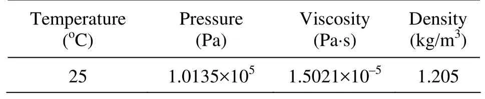
Table 1 Parameters under the numerical condition

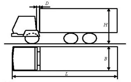
Fig.1 Diagram of numerical model

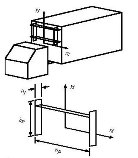
Fig.2 Sketch of fence model

(4) the airflow around a truck is steady.

A 1:10 scale truck model is built in the simulation, whose schematic view is shown in Fig.1, in which L, B and H denote the total length, the width and the height of the truck, respectively, D is the gap length between the container and the cab of the truck. A sketch of the fence installed on the truck is shown in Fig.2, where the coordinate origin is the geometrical center of the front face of the container. Four bars at the left, right, up and down positions are numbered 1 to 4, respectively. bfh, bfvand hfdenote the length, the width and the height of the fence, xfand yfare the coordinates of the fence on the front face of the container.

1.2 Mathematical model

The RNG k?ε turbulence model is used to simulate the flow field around the truck. This model differs from the standard k?ε turbulence model only in terms of the coefficients and the source[12,13], but is more suitable for a separated flow field. The air flowing around the truck can be considered as a steady turbulent fluid flow. The governing differential equations can be found in Ref.[14].

Fig.3 Sketch of the computational domain

1.3 Grids in the computational domain

According to Ref.[8], the trail region and the top region should not be smaller than five times and two times of the width of the model, respectively, for the flow field around the model not to be influenced by the boundary. So the computational domain should not be very small, but a large domain would increase the amount of computations greatly. In this article, the computational domain is 0.43 m long, 0.12 m wide and 0.09 m high. In addition to the physical model and the computational domain, the quality of the computational grids also has a crucial influence on the calculation accuracy. A fixed 3-D Cartesian coordinate system is used in the computational domain. Crosslinked structured hexahedral grids are adopted. Finer grids are employed in the regions where the flow has a sharp variation to increase the computational accuracy, and coarser grids are used where the flow is relatively uniform to reduce the CPU time. A grid pattern of 184 000 (80×50×46) nodes is used in the calculations. The rates of grid spacing variation in all sides–the front, the back and the upside of the truck are 0.7, –0.7, 0.8, –0.6, –0.6, respectively, where the negative sign means that the grid spacing enlarges toward the axis of coordinates. The grids are refined until the resultsdo not change significantly, which means that the current density of the grid sensitivity is low, the results meet our requirements. Figure 3 shows the grids in the computational domain.

1.4 Boundary conditions

Several boundary conditions are considered for the flow field around the truck: the inlet, the outlet, the walls and the computational domain profiles. When a truck is running, no boundary layer is assumed on the ground. In the wind tunnel experiments, the ground boundary layer must be eliminated, but the ground boundary cannot be removed because the truck model must be laid on a flat plate to simulate the ground in the experiments. A similar fixed floor is adopted in the calculation in order to compare the results with those obtained from the experiments. According to the model experiments and the actual flow field around the truck, the boundary conditions can be specified as follows:

For the inlet

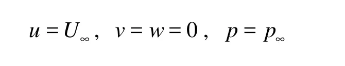
where U∞is the air velocity in the far field, and p∞is the environmental pressure. U∞=40 m/s in the experiments and the computation.

For the outlet

where the influence of the outlet section on the computational domain is neglected.

For the walls

In the computational domain, the wall boundaries, including the ground and the surface of the truck, are all non-slip boundaries, at which u = v = w =0.

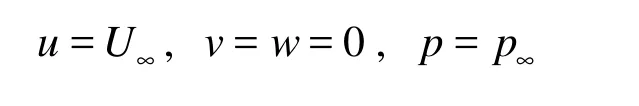
For the upside and profiles

The computational domain on the upside and the profiles of the truck are wide enough and high enough to neglect the influence of these boundaries, so u= U∞, v = w =0, p=p∞.

1.5 Numerical methods

In this article, all conservation equations and turbulence model equations are solved using the CFD software PHOENICS, based on the finite-volume method. The first-order upwind difference method is adopted for convective terms, and the central difference scheme for diffusive terms. To evaluate the pressure-velocity coupling field, the well-known SIMPLE algorithm is employed.

2. Aerodynamic drag coefficient of a truck with a hash symbol shaped fence

The velocity and the pressure in all nodes are obtained in numerical computations. In order to study the variations of the aerodynamic drag under different circumstances, the aerodynamic drag coefficients are obtained by the momentum method. Figure 4 shows a schematic diagram of the part of our study doman between the cross sections A1and A2. According to the momentum theory, the equations in the flow direction (or x direction) are as follows

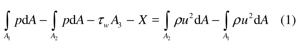
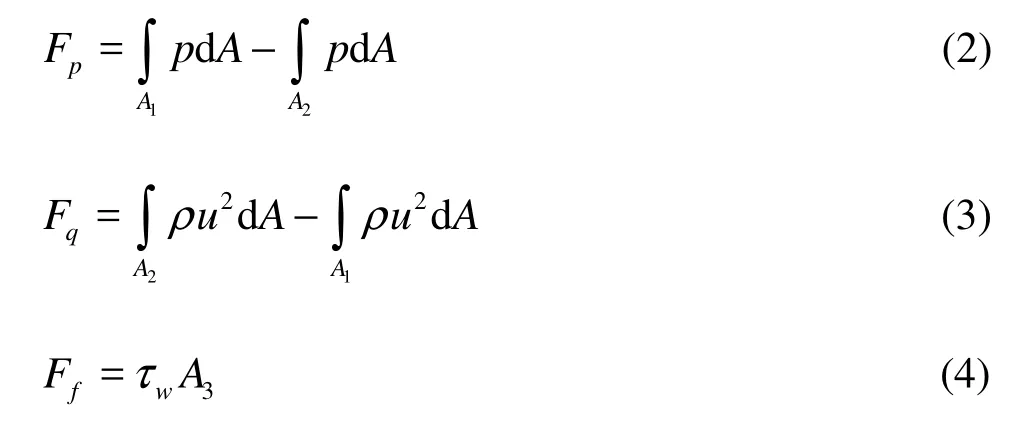
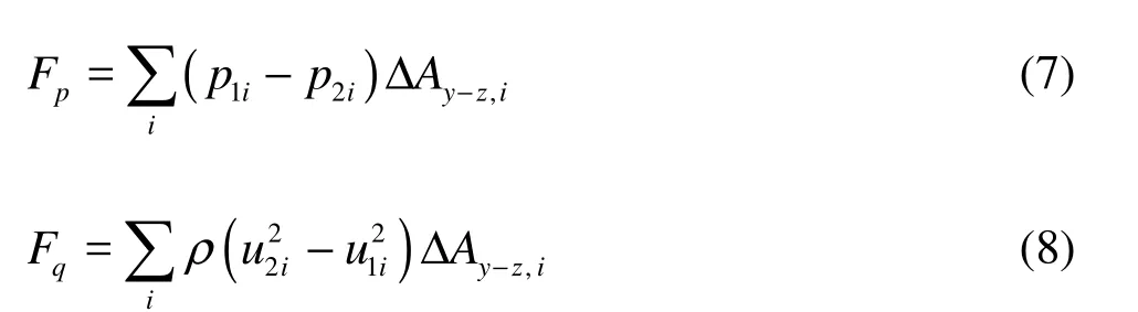
where A3=5lB and τw=0.036ρU∞2Rel?1/5is the surface friction stress. The pressure drag, the rate of change of momentum and the surface friction are Fp, Fqand Ff, respectively, are

Substituting Eqs.(9), (10) and (11) into Eq.(8), it follows that

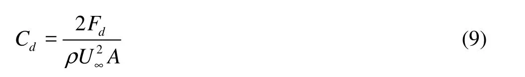
According to the resistance formula

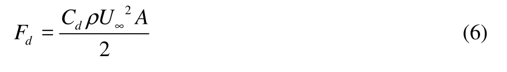
the aerodynamic drag coefficient Cdcan be obtained.

The above integral expressions, being discretized, are as follows:

Therefore, the aerodynamic drag coefficient Cdis

In the discretized equations, ΔAy?z,iis the area of the ith grid in the y-z plane, A is the sectional area perpendicular to the flow direction, the other parameters are shown in Fig.4. According to the above discretized equations, a FORTRAN program is developed to calculate the aerodynamic drag coefficients. The data of the front grid and the behind grid of the model in Fig.4 are adopted in the computation.

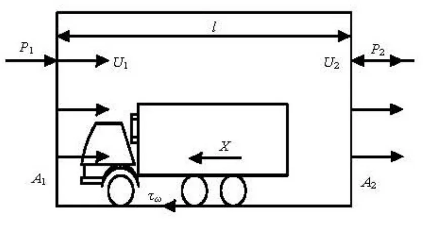
Fig.4 Model for the aerodynamic drag coefficient

3. Numerical process

In this work we take the following computation steps.

(1) First let H =0.36 m and D =0.02 m, the sizes of the hash symbol shaped fence installed on the front face of the container are bfh=0.185 m, bfv= 0.21m. Change the position and the height of the fence, until the best position and the best height is obtained.

(2) Then change the gap between the container and the cab of the truck, (D=0.03 m, 0.04 m and 0.05 m), until the best position and best height of the grid is obtained.

4. Results and discussions

4.1 Results and analysis of the computed map

From the VR-viewer of program PHOENICS, a few typical sections are used to illustrate the theory. The following section planes are all from the example of D =0.03m , hf=0.02 m , xf=0.08 m, –0.08 m, yf=0.1 m, –0.01 m. In the grid distribution, the truck is in the region of ix=18-28, iy=1-20 and iz= 16-46. The letters (a) and (b) denote the illustrative map before and after installing the hash symbol shaped fence on the truck, respectively.

From Figs.5, 6 and 7, we can see that the separating point along the flowing line moves backward after installing the hash symbol shaped fence. Before installing the hash symbol shaped fence, the separating point is at x =0.6 m. But after installing the fence, the flowing line is separated from the body at x =0.85 m . The separating point is much closer to the rear end of the truck, so the trail eddy area is reduced, and the pressure drop resistance is decreased accordingly.

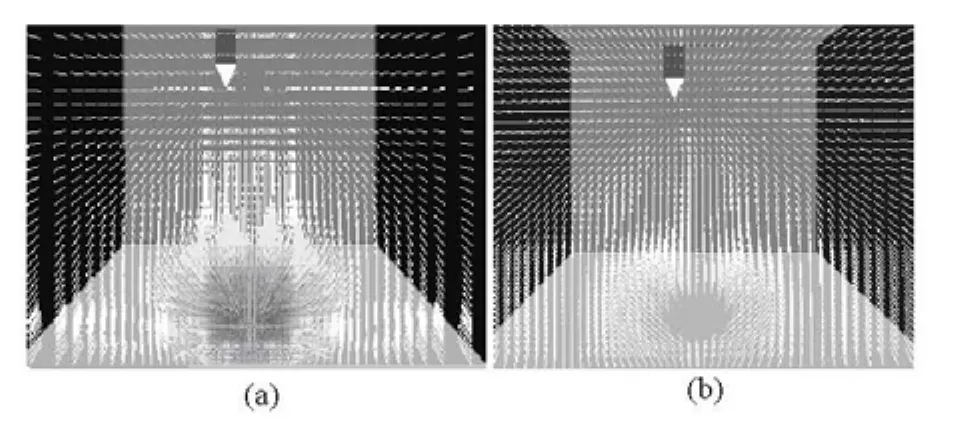
Fig.5 Sectional pressure distribution map ( z =0.55 m )

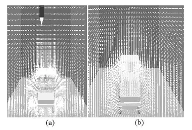
Fig.6 Sectional pressure distribution map (z=0.6 m)

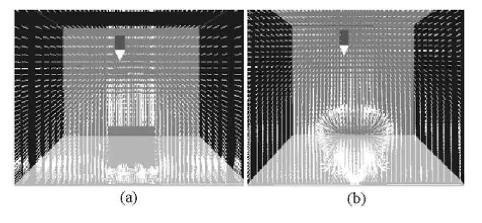
Fig.7 Sectional pressure distribution map ( z =0.85 m )

4.2 Results and analysis of aerodynamic drag coefficient

The computated aerodynamic drag coefficient results under different conditions are shown in Table 2. For different gaps, the optimal position and height of fences are illustrated in the Table 2. With the increase of the gap, the optimal size of fences increases. However, as the gap D increases to 0.05 m, the best height starts to decrease. A different gap D, a different position and a different height of the fence will lead to a different flowing map of the cab and the container. When the position and the height of the fence take optimal values, the air upward refraction angle assumes a proper value. Thus not only the air windward impinging on the container is avoided, but alsothe air separating area on the top of the container is eliminated. Under this circumstance, we will have the optimal flow field map.

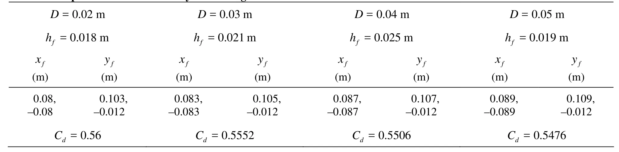
Table 2 Computated results of aerodynamic drag coefficient

5. Wind tunnel experiments on a truck with a hash symbol shaped fence

The experiments in this work are carried out in a low speed wind tunnel in Shandong University. The wind tunnel is a single return flow tunnel with a

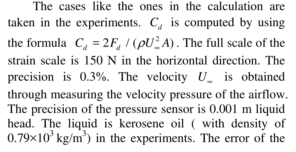
1 m×1.2 m rectangular corner, a symmetrically cut outlet, and a section area of 1.12 m2. The working section length is 2 m, the steady wind velocity is 10 m/s-40 m/s and the turbulence scale is no more than 0.3%. A silicon controlled rectifier continuously controls the speed. The 1:10 truck model in these experiments has the same dimensions as those used in the computation. As the wind speed is 40 m / s, the Reynolds number is 0.58 × 106-0.67 × 106. The model is fixed in the wind tunnel as shown in Fig.8. A strain scale measures the total resistance acting on the truck. measured area is less than 10–6m2. So, the relative deviation of Cdis about 1.12%.

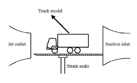
Fig.8 Model installed in the wind tunnel

The experiments are used to validate the numerical results. Change the gap D to obtain the hydrodynamic drag Fdfor different positions and different heights of the hash symbol shaped fence. With the above method, the aerodynamic drag coefficient Cdis obtained. By comparing the value with the numerical results, the inherent relation between different parameters can be obtained. In the experiments, the gap D, the height and the position of the hash symbol shaped fence hfare adjusted to validate the numerical results. To save time and expenses of the experiments, the experiments are simplified based on the numerical results. However, the results can verify the accuracy of the computations. As shown in Fig.9, the data of the experiments confirm that the simulation is reliable. The variation trends of the resistance coefficient for different gaps and different sizes of the fences are consistent with the trends of the computational results. But, the hydrodynamic drag coefficients obtained from the computation are greater than those obtained from experiments, which may be explained as in Ref.[14].

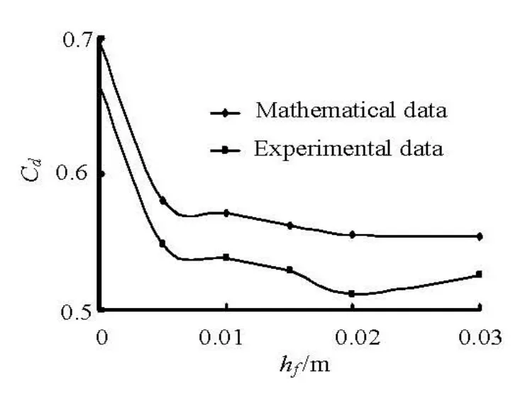
Fig.9 Curve of computed data and experimental data (D= 0.04 m)

6. Comprehensive analysis

After a comprehensive analysis of numerical and experimental results, we can see that within the scopeof this study (namely H =0.36 m , D=0.02 m-0.05 m), if the height of the container is constant, the resistance coefficient decreases with the increase of the gap size. After installing the hash symbol shaped fence, the resistance coefficients under various conditions are decreased, but the decrease extents and the best position of the fences are different. As the size of the hash symbol shaped fence increases, the Aerodynamic Drag Coefficient (ADC) increases first, then decreases. There is a minimum during this process, which is very important for drag reduction design for trucks. In the truck design, the fence should be in the best position and of the best size. Obviously after installing the hash symbol shaped fence, the flow field around the truck is improved, so the positive pressure area in the front of the truck and the negative pressure area in the rear of the truck are diminished.

For various gaps, the optimal position and height of fences are obtained in simulations and experiments. With the increase of the gap size, the optimal size of fences increases. However, as the gap D increases to a value of 0.05 m, the best height starts to decrease. After a careful analysis, it is seen that the eddy area on the top of the rear end of the cab works as a dome, which serves as a shield to the container. The size of the eddy area decides if this shield effect is sufficiently large. With different gaps D, different positions and different heights of the fence, we have different flowing maps of the cab and the container. The eddy area is smaller if without the hash symbol shaped fence, and the upward refraction of the airstream is insufficient, so a great amount of air would impinge on the container upward of cab with high speed, to form an area on the upward surface, where the air is separated. Thus, the drag coefficient would be larger. If the size and the height of the fence installed on the truck are small, the airstream is partly refracted upward, the other part of the air still impinges on the container. Under this circumstance, the drag coefficient is smaller than the above circumstances, but it is not the optimal state. For the position and the height of the fence to be in the optimal state, the air upward refraction angle should be properly chosen, not only the air windward impinging on the container is avoided, but also the air separating area on the top of the container is eliminated. Under this circumstance, we will have the optimal map. However, if the size and the height of the fence continue to increase, the eddy area on the top of the container will increase, and the air upward refraction angle will be larger. Thus, the air windward impinging area on the container would be eliminated, but a larger air separating area would appear on the top of the container, which is unfavorable to the improvement of the aerodynamic drag characteristics. So as the gap D increases to the value of 0.05 m, if the size and the height of the fence continue to increase, there will be an excessive air refraction, to increase the drag coefficient instead. The optimal height and position of the fence should be determined by experiments and calculations for different truck parameters.

7. Conclusions

According to the numerical simulation, model experiments and theoretical analysis, the following conclusions can be reached:

(1) After installing the hash symbol shaped fence on the truck, the drag reduction effects are very good. In this study, with the dimensions of H=0.36 m and D =0.03m, the drag can be reduced by 21.29%. So installing hash symbol shaped fences is a good measure to improve the truck transportation performance.

(2) Under the condition of this study, the optimal position of the fences installed on the truck is:

As the gap D =0.02 m, the minimum drag coefficient is in the area about hf=0.015 m-0.02 m, xf=0.08 m-0.09 m, yf=0.1 m, –0.01 m, 0.11 m,–0.01 m, 0.1 m, –0.02 m and 0.11 m, –0.02 m.

As the gap D =0.03m, the minimum drag coefficient is in the area about hf=0.02 m-0.03m, xf=0.08 m-0.09 m, yf=0.1 m, –0.01 m, –0.11 m,–0.01 m and 0.1 m, –0.02 m, –0.11, –0.02 m.

As the gap D =0.04 m, the minimum drag coefficient is in the area about hf=0.02 m-0.03m, xf=0.08 m-0.09 m, yf=0.1 m, –0.01 m, –0.11 m,–0.01 m and 0.1 m, –0.02 m, –0.11 m, –0.02 m.

As the gap D =0.05 m, the minimum drag coefficient is in the area about hf=0.015 m-0.02 m, xf=0.08 m-0.09 m, yf=0.1 m, –0.01 m, –0.11 m,–0.01 m and 0.1 m, –0.020 m, –0.11 m, –0.02 m.

(3) Within the scope of this simulation, with the increase of the gap D, the drag coefficient decreases gradually, the optimal size of the fences increases gradually and the optimal height of the fences increases first, then decreases.

(4) The geometry and position of the truck bodywork and the additive settings should be investigated carefully. As the bodywork changes, the optimal size and position of the fences will change accordingly. The results and analyses in this article can provide some guidance in this respect.

References

[1] MOHAMED-KASSIM Z., FILIPPONE A. Fuel savings on a heavy vehicle via aerodynamic drag reduction[J]. Transportation Research Part D: Transport and Environment, 2010, 15(5): 275-284.

[2] PAOLO F. The effect of the competition between cars and trucks on the evolution of the motorway transport system[J]. Transportation Research Part C: Emerging Technologies, 2009, 17(6): 558-570.

[3] HASSAN H., CHRIS B. Large-eddy simulation of the flow around a freight wagon subjected to a crosswind[J]. Computers and Fluids, 2010,39(10): 1944-1956.

[4] COGOTTI A. Evolution of performance of an automotive wind tunnel[J]. Journal of Wind Engineering and Industrial Aerodynamics, 2008, 96(6-7): 667-700.

[5] YAO Yan, LU Chuan-jing and SI Ting et al. Experimental investigation on the drag reduction characteristics of traveling wavy wall at high Reynolds number in wind tunnel[J]. Journal of Hydrodynamics, 2010, 22(5): 719-724.

[6] AL-GARNI A. M., BERNAL L. P. Experimental study of a pickup truck near wake[J]. Journal of Wind Engineering and Industrial Aerodynamics, 2010, 98(2): 100-112.

[7] GOHLKE M., BEAUDOIN J. F. and AMIELH M. et al. Shape influence on mean forces applied on a ground vehicle under steady cross-wind source[J]. Journal of Wind Engineering and Industrial Aerodynamics, 2010, 98(8-9): 386-391.

[8] HUANG Yuan-dong, GAO Wei and KIM Chang-Nyung. A numerical study of the train-induced unsteady airflow in a subway tunnel with natural ventilation ducts using the dynamic layering method[J]. Journal of Hydrodynamics, 2010, 22(2): 164-172.

[9] NI Chong-ben, ZHU Ren-chuan and MIAO Guo-ping et al. A method for ship resistance prediction based on CFD computation[J]. Chinese Journal of Hydrodynamics, 2010, 25(5): 579-586(in Chinese).

[10] WANG Jin-bao, YU Hai and ZHANG Yue-feng et al. Numerical simulation of viscous wake field and resistance prediction around slow-full ships[J]. Chinese Journal of Hydrodynamics, 2010, 25(5): 648-656(in Chinese).

[11] LI Li, DU Guang-sheng and LIU Zheng-gang et al. The transient aerodynamic characteristics around vans running into a road tunnel[J]. Journal of Hydrodynamics, 2010, 22(2): 283-288.

[12] TSUBOKURA M., NAKASHIMA T. and KITAYAMA M. et al. Large eddy simulation on the unsteady aerodynamic response of a road vehicle in transient crosswinds[J]. International Journal of Heat and Fluid Flow, 2010, 31(6): 1075-1086.

[13] HYAMS D. G., SREENIVAS K. and PANKAJAKSHAN R. et al. Computational simulation of model and full scale Class 8 trucks with drag reduction devices[J]. Computers and Fluids, 2011, 41(1): 27-40.

[14] QI Xiao-ni, LIU Zhen-yan. Investigation on drag reduction of trucks[J]. Journal of Shanghai Jiaotong University (Science), 2008,13(2): 201-205.

10.1016/S1001-6058(10)60173-4

* Biography: QI Xiao-ni (1974-), Female, Ph. D., Lecturer

LIU Yong-qi, E-mail: bmjw@163.com